Traveling Salesman Problem: Exact Solutions vs. Heuristic vs. Approximation Algorithms

1. Introduction

The Traveling Salesman Problem (TSP) is a well-known challenge in computer science, mathematical optimization, and operations research that aims to locate the most efficient route for visiting a group of cities and returning to the initial city. TSP is an extensively researched topic in the realm of combinatorial optimization. It has practical uses in various other optimization problems, including electronic circuit design, job sequencing, and so forth.

This tutorial will delve into the TSP definition and various types of algorithms that can be used to solve the problem. These algorithms include exact, heuristic, and approximation methods.

2. Travelling Salesman Problem

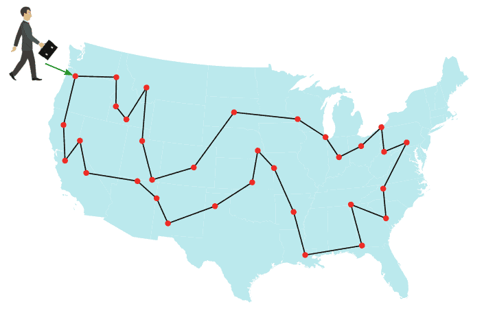
The TSP is often presented as a challenge to determine the shortest route between cities while visiting each city exactly once and returning to the starting city, using a list of cities and the distances between them. The below figures illustrate a TSP instance for several cities in the United States:

Illustration of the Travelling Saleman Problem

TSP is considered an NP-hard problem, meaning that the time required to find the optimal solution increases exponentially as the number of cities grows. Despite its complexity, the TSP is used in many practical applications, such as optimizing delivery truck routes and scheduling manufacturing processes.

3. Mathematical Formulations

The TSP can be expressed mathematically as an Integer Linear Program (ILP). There are two well-known formulations of the problem, the Miller-Tucker-Zemlin (MTZ) formulation, and the Dantzig-Fulkerson-Johnson (DFJ) formulation.

In both formulations, the cities are labeled with indices $1, \ldots, n$ . Each path from city i to city j is associated with a cost (or distance) $c_{ij}>0$ . The binary variable $x_{ij}$ indicates whether there exists a path between city $i$ and city $j$ :

$x_{ij}=\begin{cases} 1 & \text{the path goes from city }i\text{ to city }j,\\ 0 & \text{otherwise}. \end{cases}$

The objective in both formulations is to minimize the tour length,

given by

$\text{tour length}=\sum_{i=1}^{n}\sum_{j=1,j\neq i}^{n}c_{ij}x_{ij}.$

3.1. Miller–Tucker–Zemlin (MTZ) Formulation

The MTZ formulation for TSP was introduced by C. E. Miller, A. W. Tucker, and R. A. Zemlin in the Journal of ACM in 1960. This formulation includes an extra variable, $u_{i}\in\mathbb{Z}$ , which represents the order in which the cities are visited, starting from city 1. The value of $u_{i}$ indicates the position of city i in the tour, where $u_{i}<u_{j}$ implies that city $i$ is visited before city $j$ :

$\begin{align*} \text{min}\, & \sum_{i=1}^{n}\sum_{j\neq i,j=1}^{n}c_{ij}x_{ij} & \left(1\right)\\ \text{s.t.}\, & \sum_{i=1,i\neq j}^{n}x_{ij}=1,\quad j=1,\ldots,n; & \left(2\right)\\ & \sum_{j=1,j\neq i}^{n}x_{ij}=1,\quad i=1,\ldots,n; & \left(3\right)\\ & u_{i}-u_{j}+(n-1)x_{ij}\leq n-2,\quad2\leq i\neq j\leq n; & \left(4\right)\\ & 1\leq u_{i}\leq n-1,\quad2\leq i\leq n. & \left(5\right) \end{align*}$

In this formulation, constraint (1) mandates that each city must be reached from precisely one other city. Constraint (2) guarantees that from each city, there is a single departure to another city. Lastly, constraints (4) and (5) ensure that there is only one tour that covers all cities and no two or more separate tours that collectively cover all the cities. These constraints are necessary to ensure that the resulting solution is a valid tour of all cities.

3.2. Dantzig–Fulkerson–Johnson (DFJ) Formulation

The DFJ formulation for TSP was published by G. Dantzig, R. Fulkerson, and S. Johnson in the Journal of the Operations Research Society of America in 1954. Their proposed formulation is described as follows:

$\begin{align*} \text{min}\, & \sum_{i=1}^{n}\sum_{j\neq i,j=1}^{n}c_{ij}x_{ij} & \left(1\right)\\ \text{s.t.}\, & \sum_{i=1,i\neq j}^{n}x_{ij}=1,\quad j=1,\ldots,n; & \left(2\right)\\ & \sum_{j=1,j\neq i}^{n}x_{ij}=1,\quad i=1,\ldots,n; & \left(3\right)\\ & \sum_{i\in Q}\sum_{j\neq i,j\in Q}x_{ij}\leq|Q|-1,\quad\forall Q\subsetneq\{1,\ldots,n\},|Q|\geq2. & \left(4\right) \end{align*}$

Constraints (2) and (3) of the DFJ formulation are identical to those in the MTZ formulation. The last constraint (4), referred to as a subtour elimination constraint, implies that no proper subset $Q$ can form a sub-tour, ensuring that the solution obtained is a single tour rather than a combination of smaller tours. However, enforcing this constraint would lead to an enormous number of possible constraints, making it impractical to solve using traditional methods. In practice, this is solved using the row generation method.

4. TSP Algorithms

Researchers have developed several algorithms to solve the TSP, including exact, heuristic, and approximation algorithms.

Exact algorithms can find the optimal solution but are only feasible for small problem instances.

On the other hand, heuristic algorithms can handle larger problem instances but cannot guarantee to find the optimal solution.

Approximation algorithms balance speed and optimality by producing solutions that are guaranteed to be within a specific percentage of the optimal solution.

4.1. Exact Algorithms

The following table summarizes several exact algorithms to solve TSP:

	Description
Brute-force search	Approach: Try all permutations Complexity: $\mathcal{O}(n!)$ Suitable only for a small network with few cities
Held-Karp algorithm	Approach: Dynamic programming Complexity: $\mathcal{O}(n^{2}2^{n})$ Suitable for an average network with 40-60 cities
Concorde TSP solver	Approach: Branch-and-cut-and-price Can solve for a network of 85,900 cities but taking over 136 CPU-years

The simplest approach to solve the TSP is to use brute-force search, which involves trying all possible permutations of paths and selecting the shortest one. However, the running time of this method is $\mathcal{O}(n!)$ , i.e., proportional to the factorial of the number of cities, which means that it quickly becomes impractical even for small instances of the problem.

Dynamic programming is another technique that can be used to solve the TSP. One of the earliest dynamic programming algorithms for the TSP is the Held-Karp algorithm, which has a running time of $\mathcal{O}(n^{2}2^{n})$ . However, improving the time complexity beyond this point appears to be quite challenging.

More recently, Ambainis et al. proposed a quantum exact algorithm for the TSP that has a running time of $\mathcal{O}(1.728^{n})$ . This algorithm is currently the best-known algorithm for solving the TSP exactly, but it is not yet practical for solving large instances of the problem.

Other approaches include various brand-and-bound algorithms and branch-and-cut algorithms. Branch-and-bound algorithms can handle TSPs with 40-60 cities, while branch-and-cut algorithms can handle larger instances. An example is the Concorde TSP Solver, which was introduced by Applegate et al. in 2006 and can solve a TSP with almost 86,000 cities, but it requires 136 CPU years to do so.

4.2. Heuristics Algorithms

This section will discover some heuristics to solve TSP, including Match Twice and Stitch (MTS) and Lin-Kernighan heuristics. The description of these heuristics are summarized in the below table:

Algorithm	Description
Match Twice and Stitch	Approach: sequential matching Complexity: $\mathcalO(n^2)$
Lin-Kernighan	Approach: local search Complexity: $\displaystyle \mathcalO(n^\lfloor p_1/2\rfloor)$ ( $p_1$ is the backtracking depth)

The MTS heuristic consists of two phases. In the first phase, known as cycle construction, two sequential matchings are performed to construct cycles. The first matching returns the minimum-cost edge set with each point incident to exactly one matching edge. Next, all these edges are removed, and the second matching is executed. The second matching repeats the matching process, subject to the constraint that none of the edges chosen in the first matching can be used again. Together, the results of the first and second matchings form a set of cycles. The constructed cycles are stitched together in the second phase to form the TSP tour.

Lin-Kernighan is a local search algorithm and one of the most effective heuristics to solve the symmetric TSP. It takes an existing tour (Hamiltonian cycle) as input and tries to improve it by exploring the neighboring tours to find a shorter one. This process is repeated until a local minimum is reached. The algorithm uses a similar concept as 2-opt and 3-opt algorithms, where the “distance” between two tours is the number of edges that are different between them. Lin-Kernighan builds new tours by rearranging segments of the old tour, sometimes reversing the direction of traversal. It is adaptive and does not have a fixed number of edges to replace in a step, but it tends to replace a small number of edges, such as 2 or 3, at a time.

4.3. Approximation Algorithms

In this section, we’ll discuss two well-known approximation algorithms for TSP, namely the Nearest Neighbor (NN) and the Christofides-Serdyukov algorithms. The description of these algorithms are summarized in the below table:

Algorithm	Description
Nearest Neighbour (NN)	Approach: greedy search Approximation factor: $\log{\|V\|}$
Christofides-Serdyukov	Approach: combines the minimum spanning tree with minimum-weight perfect matching Approximation factor: 1.5

The NN algorithm is a greedy approach where the salesman chooses the closest unvisited city as the next destination. This method quickly produces a reasonably short route. For $n$ cities randomly located on a plane, on average, the algorithm generates a path that is 25% longer than the shortest possible path. However, some city distributions are designed explicitly to make the NN algorithm perform poorly, which is true for both symmetric and asymmetric TSPs. Researchers have shown that the NN algorithm has an approximation factor of $\log|V|$ for instances satisfying the triangle inequality.

The Christofides–Serdyukov algorithm is another approximation algorithm for the TSP that utilizes both the minimum spanning tree and a solution to the minimum-weight perfect matching problem. By combining these two solutions, the algorithm is able to produce a TSP tour that is at most 1.5 times the length of the optimal tour. This algorithm was among the first approximation algorithms and played a significant role in popularizing the use of approximation algorithms as a practical approach to solving computationally difficult problems.

5. Applications of TSP

TSP has numerous applications across different fields, including:

Logistics and supply chain management: The TSP is often used to optimize delivery routes and minimize travel costs for logistics and supply chain management. For example, companies like UPS and FedEx use TSP algorithms to optimize their delivery routes and schedules
DNA sequencing: The TSP has been used in DNA sequencing to determine the order in which to fragment a DNA molecule to obtain its complete sequence. TSP algorithms can help minimize the number of fragments required to sequence a DNA molecule
Circuit board design: TSP algorithms can be used to optimize the design of circuit boards, where the goal is to minimize the length of the connections between the components
Network design: The TSP can be used to design optimal networks for telecommunications, transportation, and other systems. The TSP can help optimize the placement of facilities and routing of traffic in such systems
Manufacturing and production planning: The TSP can be used in production planning and scheduling to optimize the order in which different tasks are performed, minimize setup times, and reduce production costs
Robotics: The TSP can be used to optimize the path of a robot as it moves through a series of tasks or objectives. TSP algorithms can help minimize the distance traveled by the robot and reduce the time required to complete the tasks
Image and video processing: The TSP can be used to optimize the order in which different parts of an image or video are processed. This can help improve the efficiency of image and video processing algorithms

6. Conclusion

TSP is a classic problem in computer science and operations research, which has a wide range of applications in various fields, from academia to industry.

This brief provides an overview of the travelling salesman problem, including its definition, mathematical formulations, and several algorithms to solve the problem, which is divided into three main categories: exact, heuristic, and approximation algorithms.

Learn Java Collections

Learn Spring

Learn Maven

View All Courses

Core Concepts

Operating Systems

Neural Networks

Graph Theory

Latex

Full Archive

About Baeldung