

Learn through the super-clean Baeldung Pro experience:
>> Membership and Baeldung Pro.
No ads, dark-mode and 6 months free of IntelliJ Idea Ultimate to start with.
Learn through the super-clean Baeldung Pro experience:
>> Membership and Baeldung Pro.
No ads, dark-mode and 6 months free of IntelliJ Idea Ultimate to start with.
Constrained optimization, also known as constraint optimization, is the process of optimizing an objective function with respect to a set of decision variables while imposing constraints on those variables.
In this tutorial, we’ll provide a brief introduction to constrained optimization, explore some examples, and introduce some methods to solve constrained optimization problems.
In a constrained optimization problem, the objective function is either a cost function (to be minimized) or a reward/utility function (to be maximized).
Now, let’s examine situations where a function is constrained. A constraint is a hard limit we place on a variable’s value to prevent the objective function from going forever in certain directions:
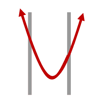
With nonlinear functions, the optima (maximum or minimum values) can either occur at the boundaries or between them:
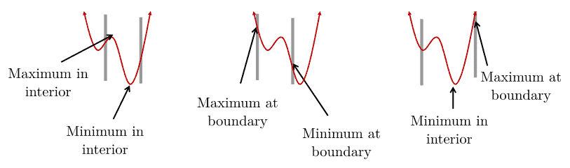
As we can see, the maximum or minimum values can occur in the interior or at boundaries.
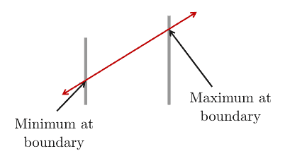
In contrast, with linear functions, the maximum or minimum values occur only at boundaries:
The following formulation describes the general (canonical) form of a constrained minimization problem:
![\[\begin{array}{rll} \mathrm{min}\, & f(\mathbf{x})\\ \mathrm{s.t.}\, & g_{i}(\mathbf{x})=c_{i} & \text{for }i=1,\ldots,n\, \text{(equality constraints)}\\ & h_{j}(\mathbf{x})\geq d_{j} & \text{for }j=1,\ldots,m\, \text{(inequality constraints)} \end{array}\]](/wp-content/ql-cache/quicklatex.com-96ee9442e8f1d5ada347680c994fe347_l3.svg "Rendered by QuickLaTeX.com")
where  is the vector of decision variables;
  is the objective function that needs to be optimized;
  for
for  and
and  for
for  are constraints that are required to be satisfied.
If we need to maximize the objective function, e.g., the utilization efficiency of network resources, we can negate it to make it fit the general form:
![\[\begin{array}{rl} \mathrm{max}\, & f(\mathbf{x})\\ \mathrm{s.t.}\, & \mathrm{constraints} \end{array}\quad\equiv\quad\begin{array}{rl} \mathrm{min}\, & -f(\mathbf{x})\\ \mathrm{s.t.}\, & \mathrm{constraints} \end{array}\]](/wp-content/ql-cache/quicklatex.com-5e38a243ace7625c97f3e33664aef1da_l3.svg "Rendered by QuickLaTeX.com")
Depending on the objective function and constraints, there are several types of constrained optimization problems.
Linear Programming (LP) covers the cases in which the objective function is linear and all constraints are also linear. If all decision variables are integers, then we’ll have an Integer Linear Programming (ILP) problem. If only some of the decision variables are integers (the remaining are continuous), that’s a Mixed Integer Linear Programming (MILP) problem.
For example:
![\[\begin{array}{rl} \mathrm{min}\, & x_{1}+2x_{2}+3x_{3}\\ \mathrm{s.t.}\, & 3x_{1}+x_{2}\geq6\\ & 7x_{1}-2x_{2}\geq1\\ & x_{1},x_{2}\in\mathbb{R}_{+} \end{array}\]](/wp-content/ql-cache/quicklatex.com-7b9e54df3f290481dfb8f18247876a61_l3.svg "Rendered by QuickLaTeX.com")
Nonlinear Programming (NLP) refers to the problems where the objective function or some constraints are nonlinear. Similar to linear programming, there are Integer Nonlinear Programming (INLP) and Mixed Integer Nonlinear Programming (MINLP).
Here’s an example of a problem with nonlinear constraints:
![\[\begin{array}{rl} \mathrm{min}\, & x_{1}+2x_{2}+3x_{3}\\ \mathrm{s.t.}\, & 3x_{1}x_{2}\geq 6\\ & 7x_{1}-2x_{2}\geq 1\\ & x_{1}, x_{2} \in \mathbb{R}_{+} \end{array}\]](/wp-content/ql-cache/quicklatex.com-9f08349a6caabd3862797c47606bbb23_l3.svg "Rendered by QuickLaTeX.com")
Finally, Quadratic Programming (QP) problems are those with linear constraints but the objective function is quadratic. Similar to linear programming and nonlinear programming problems, we also have Integer Quadratic Programming (IQP) and Mixed Integer Quadratic Programming (MIQP) problems.
For instance:
![\[\begin{array}{rl} \mathrm{min}\, & x_{1}+2x_{1}x_{2}+3x_{2}x_{3}\\ \mathrm{s.t.}\, & 3x_{1}+x_{2}\geq6\\ & 7x_{1}-2x_{2}\geq1\\ & x_{1},x_{2}\in\mathbb{R}_{+} \end{array}\]](/wp-content/ql-cache/quicklatex.com-c3380ae5c29e00bd7e7690a8b9d0bebd_l3.svg "Rendered by QuickLaTeX.com")
Now let’s see how we can apply constrained optimization to real-world problems. Let’s suppose we want to maximize the area of a rectangle while keeping its perimeter equal to a predefined value  :
:
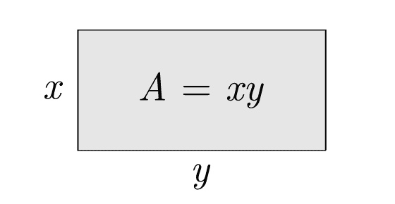
As we see, the area is  , and that will be our objective function. Further, since the perimeter needs to be equal to , we have a constrained optimization problem:
![\[\begin{array}{rl} \mathrm{max}\, & A=xy\\ \mathrm{s.t.}\, & 2(x+y)=p \end{array}\]](/wp-content/ql-cache/quicklatex.com-8e77e82ad2e142bf31b2ea51e98f628a_l3.svg "Rendered by QuickLaTeX.com")
This problem has a quadratic objective function ( ) and a linear constraint, so it falls into the QP category.
Let’s now see how we can solve constrained optimization problems.
There is, unfortunately, no universal method for solving all types of optimization problems.
Different proposed methods are tailored to particular types of optimization problems. The following table lists some classical mathematical methods for solving constrained optimization problems:
| Method | Pros | Cons | |
|---|---|---|---|
| Equality constraints | Substitution method | Easy to understand, simple to calculate | May fail when dealing with nonlinear constraints, or discontinuous objective function |
| Lagrange multiplier | Can solve NLP with complex and inequality constraints. | Must be altered to compensate for inequality constraints. Only practical for small problems | |
| Branch-and-bound algorithms | Lower complexity compared to other algorithms | Time-consuming, difficult to apply parallelization | |
| Simplex method | Memory efficient, numerically stable, high iteration speed | Not so good for large problems, difficult to apply parallelization | |
| Interior-point method | Require few iterations, easy to parallelize | Not suitable when needing a quick and degenerate basic solution | |
| Inequality constraints | Ellipsoid method (for QP) | Polynomial-time solvability for LPs | Numerical instability and poor performance in practice |
| Karush–Kuhn–Tucker (KKT) approach (for NLP) | Useful (and necessary) for checking the optimality of a solution | Not sufficient if the objective function is non-convex |
Most of these methods, such as the branch-and-bound algorithm, are exact. Exact optimization techniques are guaranteed to find the optimal solution. The price for such guarantees is that they can take a lot of time to complete. In contrast, inexact methods don’t guarantee finding the optimum but usually produce a sufficiently good solution quickly. Metaheuristics such as the Grey-Wolf Optimization algorithm fall into the category of inexact methods and are frequently used when we need to find any solution quickly.
Let’s explain the substitution method using a simple example with an equality constraint:
![\[\begin{array}{rl} \mathrm{max}\, & f(x,y)=xy\\ \mathrm{s.t.}\, & x+y=2 \end{array}\]](/wp-content/ql-cache/quicklatex.com-f477bf8a6e09946204580d08a732d58b_l3.svg "Rendered by QuickLaTeX.com")
As we see, that’s the same problem as in the above example with a rectangle. The only difference is that here, isn’t a free parameter but a known value  :
:
![\[x + y = 2 \iff 2(x + y) = 4\]](/wp-content/ql-cache/quicklatex.com-4a462b4f76e35c9b90ddb81fde44d1ea_l3.svg "Rendered by QuickLaTeX.com")
Since we have a simple equality constraint, we can use the substitution method. We use this method mostly for problems with an equality constraint from which it’s easy to express one variable in terms of others. If we’re lucky, we can substitute the variable in the objective function and get a form that isn’t hard to solve by hand.
In our example, the constraint gives us a simple substitution:
![\[y=2-x\]](/wp-content/ql-cache/quicklatex.com-e83dfe6faa465c7b4e79392ccf4ba877_l3.svg "Rendered by QuickLaTeX.com")
As a result, we can rewrite the objective function:
![\[f(x,y)=f(x)=x(2-x)=2x-x^{2}\]](/wp-content/ql-cache/quicklatex.com-82b3bb9c216d75878ebc96f198b0f5d4_l3.svg "Rendered by QuickLaTeX.com")
The maximum value of  should satisfy the first-order derivative condition:
![\[f'(x)=0\iff 2-2x=0\iff x=1\]](/wp-content/ql-cache/quicklatex.com-052490033ea8e19faf94fd6fc6ae8f3a_l3.svg "Rendered by QuickLaTeX.com")
Consequently,  , and the maximum value of
  is
is  .
.
The following table summarizes some well-known software tools for constrained optimization problems:
| Solvers | Description | Supported interface |
|---|---|---|
| CPLEX | For general purposes. The toolbox includes solvers for LP, ILP, MILP, convex and non-convex QP problems, etc. | C++, C#, Java, MATLAB, Python |
| GPLK | For LP, MIP and other related problems | C, Java |
| Gurobi | For general purposes, including solvers for LP, ILP, MILP, MIQP, etc. | C, C++, .NET, Java, MATLAB, Python, R, AMPL, C, C++, Java, MATLAB, Python, R |
| lp_solve | For MILP problems | MATLAB, Octave, Python, R, etc. |
| MATLAB, Optim. Toolbox | For general purposes, including solvers for LP, ILP, MILP, etc. | MATLAB |
| SCIP | For MIP problems | AMPL, C, C++, Java, MATLAB, Python |
They all perform built-in exact methods (e.g., simplex) and usually combine them with inexact algorithms to reach a solution faster. For instance, CPLEX uses a node heuristic along with the branch-and-cut algorithm.
In this article, we covered the principles of constrained optimization. There are several types of constrained optimization problems and many methods for solving them. Which one is the best depends on the particular problem at hand.