Combinatorial Optimization

1. Overview

Combinatorial Optimization Problems (COP) apply to a lot of interesting problems with real-world impacts. In this tutorial, we’ll learn about major problems and their solutions. Also, we’ll understand their difficulty level with a detailed example of a popular COP in the field of computer science.

2. Identification of COP

COP is the process of finding an optimal solution through the evaluation of a finite and fixed number of combinations. Mostly, they are modeled by graph theory or linear programming.

COP appears in several applications such as delivering goods to clients, finding the shortest path, assigning tasks to workers, etc. They help us increase efficiency by reducing cost and time.

Let’s show some models used to simplify and formalize real-world problems:

• Minimum Spanning Tree (MST): Given a connected and undirected graph , a spanning tree is a subgraph of that connects all the vertices. An MST has a weight less than or equal to that of every other spanning tree.
• Traveling Salesman Problem (TSP): This is a classical problem, yet a popular one in mathematics, operations research, and optimization. We’ll explain it further and give a concrete example in the next section.
• Knapsack problem: The problem often arises in resource allocation where there are financial constraints. It is studied in fields such as computer science, complexity theory, cryptography, and applied mathematics.

3. TSP: A Difficult Problem to Solve

The original problem involves a traveling salesman who must visit several cities. The question is which order to visit the cities to make the shortest possible trip. Particularly, the salesman must visit each of the cities once and then return to the original position. Following, we’ll give the mathematical model of TSP and show a concrete example.

3.1. Formal Definition

Usually, we use a graph to model the TSP problem. , with , is the set of vertices representing the cities, while is the set of edges representing the distance between each pair of cities:

3.2. Example

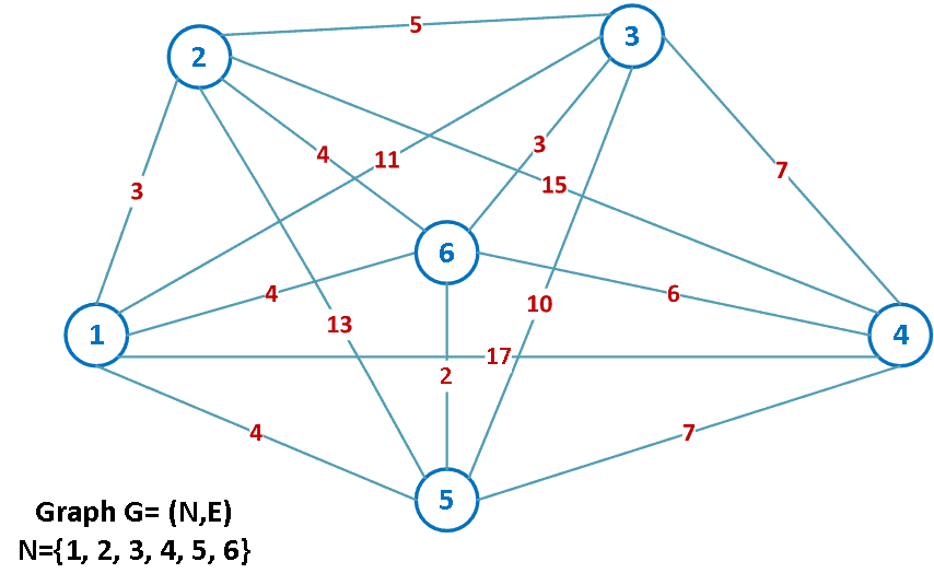
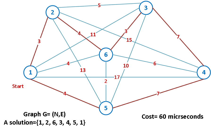
Let’s take a TSP example with a relatively small number . We assume the computer takes one unit of time to compute a solution. That is a microsecond (ms) per trajectory.

To go through each possible solution and take the best one, we need to compute candidate solutions. In our case, it’ll be and will take a computation time of 60 ms:

However, let’s say we have . Then the exploration of the search space will take 19 centuries. Clearly, it is a very huge amount of time. In fact, the factorial scales very bad in complexity computation:

We’ll examine in the next section the possible methods to resolve COP.

4. Solutions for COP

As we have seen previously with TSP, COPs are not always easy to solve. The number of possible solutions is usually huge and requires an exhaustive search through the solution space. That is why COPs are computationally expensive. They belong to the NP-hard category of problems. Usually, we tend to find a near-optimal solution in a reasonable time.

We cite two major approaches to solving COPs:

1. Exact solutions: They guarantee to obtain the global optimum. However, they take too long and have high complexity costs. They are only suitable for small-size problems. Examples are Branch and Bound algorithms, and dynamic programming.
2. Approximative solutions: They rely on a trade-off: finding an approximative solution yet a very fast one. They allow us to tackle large-size problems. Generally, they are divided into problem-specific heuristics and metaheuristics.

5. Conclusion

To sum up, in this tutorial, we’ve defined COPs and explained their level of difficulty as well as the possible solutions.