

Learn through the super-clean Baeldung Pro experience:
>> Membership and Baeldung Pro.
No ads, dark-mode and 6 months free of IntelliJ Idea Ultimate to start with.
Last updated: March 18, 2024
Learn through the super-clean Baeldung Pro experience:
>> Membership and Baeldung Pro.
No ads, dark-mode and 6 months free of IntelliJ Idea Ultimate to start with.
In computer science, there exist several famous unresolved problems, and  is one of the most studied ones. Until now, the answer to that problem is mainly “no”. And, this is accepted by the majority of the academic world. We probably wonder why this problem is still not resolved.
In this tutorial, we explain the details of this academic problem. Moreover, we also show both  and
and  problems. Then, we also add definitions of
  and
and  . And in the end, hopefully, we would have a better understanding of why is still an open problem.
To explain , , and others, let’s use the same mindset that we use to classify problems in real life. While we could use a wide range of terms to classify problems, in most cases we use an “Easy-to-Hard” scale.
Now, in theoretical computer science, the classification and complexity of common problem definitions have two major sets; which is “Polynomial” time and which “Non-deterministic Polynomial” time. There are also and sets, which we use to express more sophisticated problems. In the case of rating from easy to hard, we might label these as “easy”, “medium”, “hard”, and finally “hardest”:


And we can visualize their relationship, too: 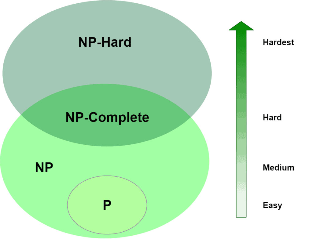
Using the diagram, we assume that and are not the same set, or, in other words, we assume that  . This is our apparently-true, but yet-unproven assertion. Of course, another interesting aspect of this diagram is that we’ve got some overlap between and . We call when the problem belongs to both of these sets.
Alright, so, we’ve mapped , , and to “easy”, “medium”, “hard” and “hardest”, but how does we place a given algorithm in each category? For that, we’ll need to get a bit more formal through the next section.
Through the rest of the article, we generally prefer not to use units like “seconds” or “milliseconds”. Instead, we prefer proportional expressions like  ,
,  ,
,  , and
, and  , using Big-O notation. Those mathematical expressions give us a clue about the algorithmic complexity of a problem.
Let’s quickly review some common Big-O values:
 – constant-time
 – logarithmic-time
 – linear-time
 – quadratic-time
 – polynomial-time
 – exponential-time
 – factorial-time
where  is a constant and is the input size. The size of also depends on the problem definition. For example, using a number set with a size of , the search problem has an average complexity between linear-time and logarithmic-time depending on the data structure in use.
The first set of problems are polynomial algorithms that we can solve in polynomial time, like logarithmic, linear or quadratic time. If an algorithm is polynomial, we can formally define its time complexity as:
 where
where  and
and  where
where  and are constants and is input size. In general, for polynomial-time algorithms
  is expected to be less than
  . Many algorithms complete in polynomial time:
As we talked about earlier, all of these have a complexity of for some , and that fact places them all in . Of course, we don’t always have just one input, . But, so long as each input is a polynomial, multiplying them will still be a polynomial. For example, in graphs, we use  for edges and
  for vertices, which gives us
  for Bellman-Ford’s shortest path algorithm. Even if the size of the edge set is
  , the time complexity is still a polynomial,
  , so we’re still in .
We can’t always pinpoint the Big-O for an algorithm. Outside of Big-O, we can think about the problem description. Consider, for example, the game of checkers. What is the complexity of determining the optimal move on a given turn? If we constrain the size of the board to  , then this is believed to be a polynomial-time problem, placing it in . But if we say it’s an
  board, it’s no longer in . In this case, how we constrain the search space affects where we place it. Similarly, the Hamiltonian-Path problem has polynomial-time solutions for only some types of input graphs.
Or another example is the stable roommate problem; it’s polynomial-time to match without a tie, but not when ties are allowed or when we include roommate preferences like married couples. (These variants are actually , which we’ll cover in a moment.) Still another factor to consider is the size of relative to . If the input size is going to be near , then the algorithm is going to behave more like an exponential.
The second set of problems cannot be solved in polynomial time. However, they can be verified (or certified) in polynomial time. We expect these algorithms to have an exponential complexity, which we’ll define as:  where
where  ,
,  and where
  ,
,  and are constants and is the input size.
  is a function of exponential-time when at least
  and
and  . As a result, we get . For example, we’ll see complexities like
  ,
,  ,
,  in this set of problems. There are several algorithms that fit this description. Among them are:
Both of these have two important characteristics: Their complexity is for some and their results can be verified in polynomial time. Those two facts place them all in , that is, the set of “Non-deterministic Polynomial” algorithms. Now, formally, we also state that these problems must be decision problems – have a yes or no answer – though note that practically speaking, all function problems can be transformed into decision problems. This distinction helps us to nail down what we mean by “verified”.
To speak precisely, then, an algorithm is in if it can’t be solved in polynomial time and the set of solutions to any decision problem can be verified in polynomial time by a “Deterministic Turing Machine“. What makes Integer Factorization and Graph Isomorphism interesting is that while we believe they are in , there’s no proof of whether they are in and . Normally, all algorithms are in , but they have another property that makes them more complex compared to problems.
Let’s continue with that difference in the next section.
The next set is very similar to the previous set. Taking a look at the diagram, all of these all belong to , but are among the hardest in the set. Right now, there are more than 3000 of these problems, and the theoretical computer science community populates the list quickly. What makes them different from other problems is a useful distinction called completeness. For any problem that’s complete, there exists a polynomial-time algorithm that can transform the problem into any other -complete problem. This transformation requirement is also called reduction.
As stated already, there are numerous problems proven to be complete. Among them are:
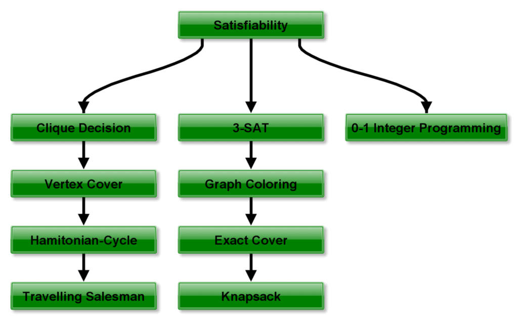
Curiously, what they have in common, aside from being in , is that each can be reduced into the other in polynomial time. These facts together place them in . The major and primary work of  belongs to Karp. And his
  problems are fundamental to this theoretical computer science topics. These works are founded on the Cook-Levin theorem and prove that the Satisfiability (SAT) problem is :
Our last set of problems contains the hardest, most complex problems in computer science. They are not only hard to solve but are hard to verify as well. In fact, some of these problems aren’t even decidable. Among the hardest computer science problems are:
These algorithms have a property similar to ones in – they can all be reduced to any problem in . Because of that, these are in and are at least as hard as any other problem in . A problem can be both in and , which is another aspect of being .
This characteristic has led to a debate about whether or not Traveling Salesman is indeed . Since and problems can be verified in polynomial time, proving that an algorithm cannot be verified in polynomial time is also sufficient for placing the algorithm in .
A question that’s fascinated many computer scientists is whether or not all algorithms in belong to : 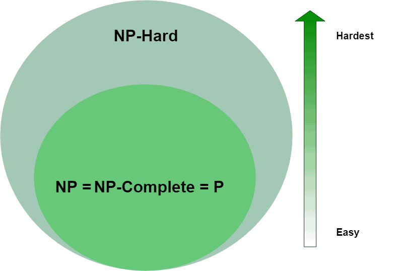 It’s an interesting problem because it would mean, for one, that any or problem can be solved in polynomial time. So far, proving that
  as proven elusive. Because of the intrigue of this problem, it’s one of the Millennium Prize Problems for which there is a $1,000,000 prize.
For our definitions, we assumed that , however,  may be possible. If it were so, aside from or problems being solvable in polynomial time, certain algorithms in would also dramatically simplify. For example, if their verifier is or
  , then it follows that they must also be solvable in polynomial time, moving them into
  as well.
We can conclude that means a radical change in computer science and even in the real-world scenarios. Currently, some security algorithms have the basis of being a requirement of too long calculation time. Many encryption schemes and algorithms in cryptography are based on the number factorization which the best-known algorithm with exponential complexity. If we find a polynomial-time algorithm, these algorithms become vulnerable to attacks.
Within this article, we have an introduction to a famous problem in computer science. Through the article, we focused on the different problem sets; , , , and . We also provided a good starting point for future studies and what-if scenarios when . Briefly after reading, we can conclude a generalized classification as follows:
problems are quick to solve problems are quick to verify but slow to solve problems are also quick to verify, slow to solve and can be reduced to any other problem problems are slow to verify, slow to solve and can be reduced to any other problemAs a final note, if has proof in the future, humankind has to construct a new way of security aspects of the computer era. When this happens, there has to be another complexity level to identify new hardness levels than we have currently.