

Learn through the super-clean Baeldung Pro experience:
>> Membership and Baeldung Pro.
No ads, dark-mode and 6 months free of IntelliJ Idea Ultimate to start with.
Learn through the super-clean Baeldung Pro experience:
>> Membership and Baeldung Pro.
No ads, dark-mode and 6 months free of IntelliJ Idea Ultimate to start with.
In computer science, there is a large number of optimization problems which has a finite but extensive number of feasible solutions. Among these, some problems like finding the shortest path in a graph or Minimum Spanning Tree can be solved in polynomial time.
A significant number of optimization problems like production planning, crew scheduling can’t be solved in polynomial time, and they belong to the NP-Hard class. These problems are the example of NP-Hard combinatorial optimization problem.
Branch and bound (B&B) is an algorithm paradigm widely used for solving such problems.
In this tutorial, we’ll discuss the branch and bound method in detail.
Branch and bound algorithms are used to find the optimal solution for combinatory, discrete, and general mathematical optimization problems. In general, given an NP-Hard problem, a branch and bound algorithm explores the entire search space of possible solutions and provides an optimal solution.
A branch and bound algorithm consist of stepwise enumeration of possible candidate solutions by exploring the entire search space. With all the possible solutions, we first build a rooted decision tree. The root node represents the entire search space:
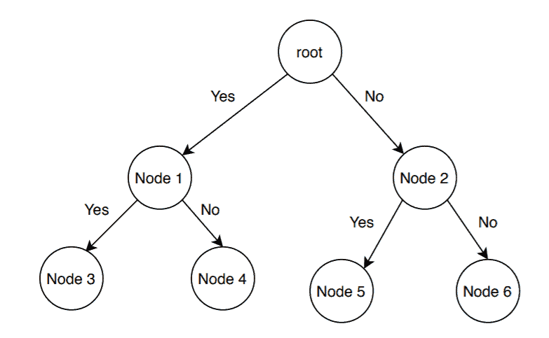
Here, each child node is a partial solution and part of the solution set. Before constructing the rooted decision tree, we set an upper and lower bound for a given problem based on the optimal solution. At each level, we need to make a decision about which node to include in the solution set. At each level, we explore the node with the best bound. In this way, we can find the best and optimal solution fast.
Now it is crucial to find a good upper and lower bound in such cases. We can find an upper bound by using any local optimization method or by picking any point in the search space. On the other hand, we can obtain a lower bound from convex relaxation or duality.
In general, we want to partition the solution set into smaller subsets of solution. Then we construct a rooted decision tree, and finally, we choose the best possible subset (node) at each level to find the best possible solution set.
We already mentioned some problems where a branch and bound can be an efficient choice over the other algorithms. In this section, we’ll list all such cases where a branch and bound algorithm is a good choice.
If the given problem is a discrete optimization problem, a branch and bound is a good choice. Discrete optimization is a subsection of optimization where the variables in the problem should belong to the discrete set. Examples of such problems are 0-1 Integer Programming or Network Flow problem.
Branch and bound work efficiently on the combinatory optimization problems. Given an objective function for an optimization problem, combinatory optimization is a process to find the maxima or minima for the objective function. The domain of the objective function should be discrete and large. Boolean Satisfiability, Integer Linear Programming are examples of the combinatory optimization problems.
In this section, we’ll discuss how the job assignment problem can be solved using a branch and bound algorithm.
Let’s first define a job assignment problem. In a standard version of a job assignment problem, there can be  jobs and workers. To keep it simple, we’re taking
  jobs and workers in our example:
| Job 1 | Job 2 | Job 3 | |
|---|---|---|---|
| A | 9 | 3 | 4 |
| B | 7 | 8 | 4 |
| C | 10 | 5 | 2 |
We can assign any of the available jobs to any worker with the condition that if a job is assigned to a worker, the other workers can’t take that particular job. We should also notice that each job has some cost associated with it, and it differs from one worker to another.
Here the main aim is to complete all the jobs by assigning one job to each worker in such a way that the sum of the cost of all the jobs should be minimized.
Now let’s discuss how to solve the job assignment problem using a branch and bound algorithm.
Let’s see the pseudocode first:
algorithm MinCost(M):
    // INPUT
    //    M = The cost matrix
    // OUTPUT
    //    The optimal job assignment minimizing the total cost

    while true:
        E <- LeastCost()
        if E is a leaf node:
            print(E)
            return
        for each child S of E:
            Add(S)
            S.parent <- E
Here,  is the input cost matrix that contains information like the number of available jobs, a list of available workers, and the associated cost for each job. The function
  maintains a list of active nodes. The function
  calculates the minimum cost of the active node at each level of the tree. After finding the node with minimum cost, we remove the node from the list of active nodes and return it.
We’re using the  function in the pseudocode, which calculates the cost of a particular node and adds it to the list of active nodes.
In the search space tree, each node contains some information, such as cost, a total number of jobs, as well as a total number of workers.
Now let’s run the algorithm on the sample example we’ve created:
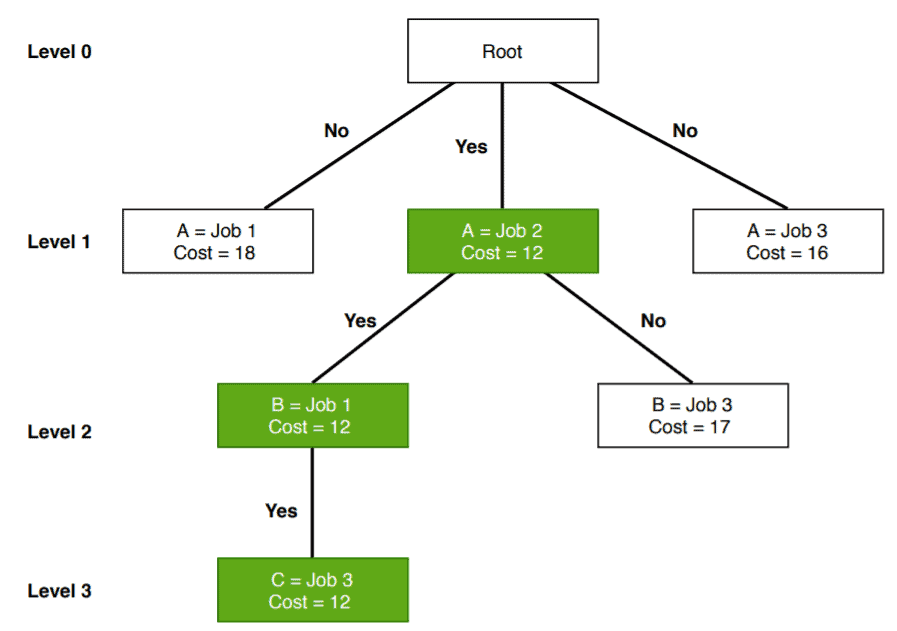
Initially, we’ve  jobs available. The worker
  has the option to take any of the available jobs. So at level
  , we assigned all the available jobs to the worker and calculated the cost. We can see that when we assigned jobs
  to the worker , it gives the lowest cost in level of the search space tree. So we assign the job
  to worker and continue the algorithm. “Yes” indicates that this is currently optimal cost.
After assigning the job to worker , we still have two open jobs. Let’s consider worker  now. We’re trying to assign either job or to worker to obtain optimal cost.
Either we can assign the job or to worker . Again we check the cost and assign job  to worker as it is the lowest in level .
Finally, we assign the job  to worker
  , and the optimal cost is
  .
.
In a branch and bound algorithm, we don’t explore all the nodes in the tree. That’s why the time complexity of the branch and bound algorithm is less when compared with other algorithms.
If the problem is not large and if we can do the branching in a reasonable amount of time, it finds an optimal solution for a given problem.
The branch and bound algorithm find a minimal path to reach the optimal solution for a given problem. It doesn’t repeat nodes while exploring the tree.
The branch and bound algorithm are time-consuming. Depending on the size of the given problem, the number of nodes in the tree can be too large in the worst case.
Also, parallelization is extremely difficult in the branch and bound algorithm.
One of the most popular algorithms used in the optimization problem is the branch and bound algorithm. We’ve discussed it thoroughly in this tutorial.
We’ve explained when a branch and bound algorithm would be the right choice for a user to use. Furthermore, we’ve presented a branch and bound based algorithm for solving the job assignment problem.
Finally, we mentioned some advantages and disadvantages of the branch and bound algorithm.