

Learn through the super-clean Baeldung Pro experience:
>> Membership and Baeldung Pro.
No ads, dark-mode and 6 months free of IntelliJ Idea Ultimate to start with.
Last updated: February 12, 2025
Learn through the super-clean Baeldung Pro experience:
>> Membership and Baeldung Pro.
No ads, dark-mode and 6 months free of IntelliJ Idea Ultimate to start with.
Reinforcement Learning (RL) has recently received considerable attention due to its successful application in several fields, including game theory, operations research, combinatorial optimization, information theory, simulation-based optimization, control theory, and statistics.
In this tutorial, we’ll explore the concept of reinforcement learning, Q-learning, deep Q-learning vs. deep Q-network, and how they relate to each other.
Reinforcement learning (RL) is a subset of machine learning in which an agent learns to obtain the best strategy for achieving its goals by interacting with the environment. Unlike supervised machine learning algorithms, which rely on ingesting and processing data, RL does not require data to learn. Instead, the agent learns from its interactions with the environment and the rewards it receives to make better decisions. In RL, the goal is to maximize the cumulative reward over time, and the agent learns through trial and error to select actions that lead to the highest rewards.
The below figure illustrates how the agent interacts with the environment in reinforcement learning:
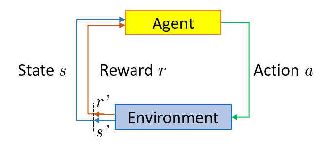
To illustrate, consider the Mario video game. If the game character takes a random action, such as moving left, it may receive a reward based on that action. After taking action, the game character (Mario) will be in a new state, and the process will repeat until Mario reaches the end of the stage or loses the game. This episode will repeat several times until Mario learns to navigate the environment by maximizing the rewards. Through this trial and error process, Mario will learn which actions lead to higher rewards and will adjust its strategy accordingly to achieve the goal of completing the level.
In brief, RL is the science of using experiences to make optimal decisions. The process involves the following simple steps:
RL algorithms can be broadly categorized into two types: model-based and model-free.
A model-based algorithm estimates the optimal policy using the transition and reward functions. In other words, it learns a model of the environment’s dynamics and uses it to predict future states and rewards.
On the other hand, a model-free algorithm does not use or estimate the environment’s dynamics. Instead, it directly estimates the optimal policy through trial and error, using the rewards received from the environment to guide its decisions. This makes model-free algorithms more suitable for environments with complex dynamics where it is difficult to model the environment accurately.
Q-learning is a model-free, value-based, off-policy algorithm that is used to find the optimal policy for an agent in a given environment. The algorithm determines the best series of actions to take based on the agent’s current state. The “Q” in Q-learning stands for quality, representing how valuable action maximizes future rewards.
As a model-based algorithm, Q-learning does not require knowledge of the transition and reward functions. It directly estimates the optimal policy through trial and error, using the rewards received from the environment to guide its decisions. The algorithm updates the Q-values based on the reward received for a particular (state, action) pair and the estimated value of the next state. By repeatedly updating the Q-values based on the observed rewards, Q-learning can converge to an optimal policy that maximizes the cumulative reward over time.
As a value-based algorithm, Q-learning trains the value function to learn which actions are more valuable in each state and select the optimal action accordingly. The value function is updated iteratively based on the rewards received from the environment, and through this process, the algorithm can converge to an optimal policy that maximizes the cumulative reward over time.
As an off-policy algorithm, Q-learning evaluates and updates a policy that differs from the policy used to take action. Specifically, Q-learning uses an epsilon-greedy policy, where the agent selects the action with the highest Q-value with probability 1-epsilon and selects a random action with probability epsilon. This exploration strategy ensures that the agent explores the environment and discovers new (state, action) pairs that may lead to higher rewards.
The Q-values are updated based on the rewards received for the action taken, even if it is not the optimal action according to the current policy. By updating the Q-values based on the highest Q-value action in each state, Q-learning can converge to the optimal policy even if it is different from the policy used to take actions during training.
As the agent exposes itself to the environment and receives different rewards by executing different actions, the values are updated per the following equation:
![\[Q_{\text{new}}\left(s,a\right)=Q\left(s,a\right)+\alpha\left(R\left(s,a\right)+\gamma\max_{a}Q'\left(s',a'\right)-Q\left(s,a\right)\right),\]](/wp-content/ql-cache/quicklatex.com-0b96d840dd73d1807257984372a03aef_l3.svg "Rendered by QuickLaTeX.com")
where  is the current Q-value,
  is the update Q-value,
  is the learning rate,
  is the reward,
  is a number between
 ![[0,1]](/wp-content/ql-cache/quicklatex.com-4ddc1168784a8b723604919df78ae658_l3.svg "Rendered by QuickLaTeX.com") and is used to discount the reward as the time passes, given the assumption that action in the beginning, is more important than at the end (an assumption that is confirmed by many real-life use cases).
and is used to discount the reward as the time passes, given the assumption that action in the beginning, is more important than at the end (an assumption that is confirmed by many real-life use cases).
In its simplest form, Q-values is a table (or matrix) with states as rows and actions as columns. The Q-table is initialized randomly, and the agent starts to interact with the environment and measures the reward for each action. It then computes the observed Q-values and updates the Q-table. The following pseudocode summarizes how Q-learning works:

Let’s see a simple example below to see how Q-learning works. Our agent is a rat that has to cross a maze and reach the end (its house) point. There are mines in the maze, and the rat can only move one tile (from one square to one another) at a time. If the rat steps onto a mine, it will be dead. The rat wants to reach its home in the shortest time possible:
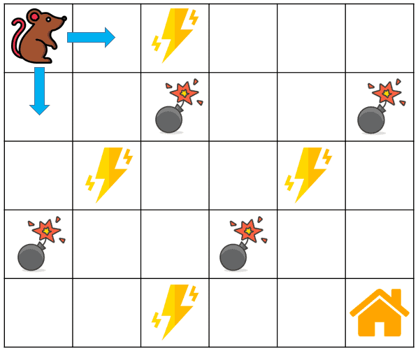
The reward system is as below:
 point
pointThe rat has four possible actions at each non-edge tile: ( ,
,  ,
,  , or
, or  ) (move up, down, right, or left). The state is the position of the rat in the maze.
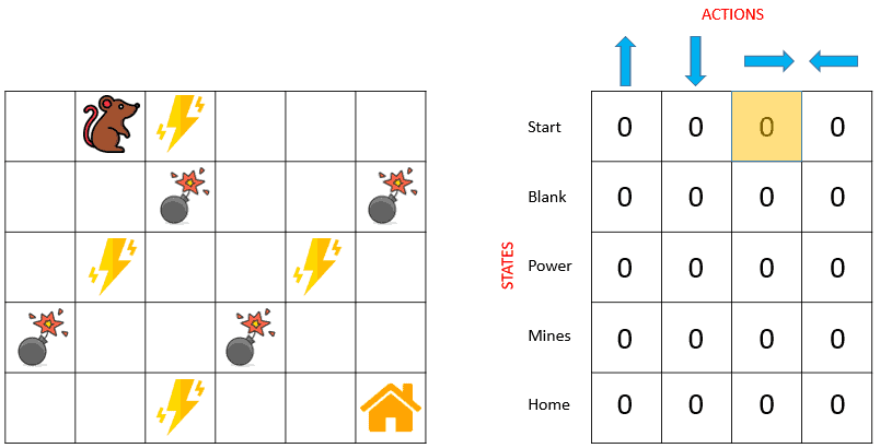
Having all this information, we can initialize the Q-table as a matrix of size 5 4, where the rows represent the rat’s possible states (positions), and the columns represent the possible actions (moving in 4 directions). Initially, our rat knows nothing about the environment (maze), so it will choose a random action, say our robot knows nothing about the environment. So the robot chooses a random action, say right:
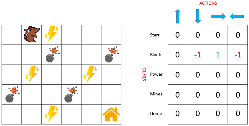
Using the Bellman equation, we can now update the Q-values for being at the start and moving right. We will repeat this again and again until the learning is stopped. In this way, the Q-table will be updated. For instance, the next Q-table corresponding to the current position of the rat looks like this:
One of the main drawbacks of Q-learning is that it becomes infeasible when dealing with large state spaces, as the size of the Q-table grows exponentially with the number of states and actions. In such cases, the algorithm becomes computationally expensive and requires a lot of memory to store the Q-values. Imagine a game with 1000 states and 1000 actions per state. We would need a table of one million cells. And that is a very small state space compared to chess or Go. Also, Q-learning can’t be used in unknown states because it can’t infer the Q-value of new states from the previous ones. This presents two problems:
First, the amount of memory required to save and update that table would increase as the number of states increases.
Second, the amount of time required to explore each state to create the required Q-table would be unrealistic.
To tackle this challenge, one alternative approach is to combine Q-learning with deep neural networks. This approach is coined as Deep Q-Learning (DQL). The neural networks in DQL act as the Q-value approximator for each (state, action) pair.
The neural network receives the state as an input and outputs the Q-values for all possible actions. The following figure illustrates the difference between Q-learning and deep Q-learning in evaluating the Q-value:
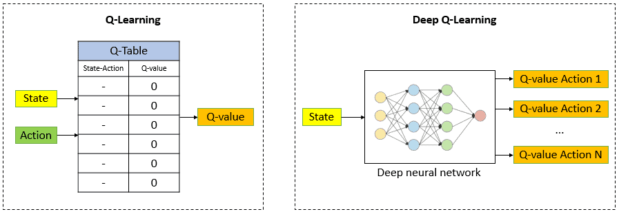
Essentially, deep Q-Learning replaces the regular Q-table with the neural network. Rather than mapping a (state, action) pair to a Q-value, the neural network maps input states to (action, Q-value) pairs.
In 2013, DeepMind introduced Deep Q-Network (DQN) algorithm. DQN is designed to learn to play Atari games from raw pixels. This was a breakthrough in the field of reinforcement learning and helped pave the way for future developments in the field. The term Deep Q-network refers to the neural network in their DQL architecture.
Here are the steps of how DQN works:
In summary, DQN learns the optimal policy by using a deep neural network to estimate the Q-values, a replay memory buffer to store past experiences, and a target network to prevent overestimating Q-values. The agent uses an epsilon-greedy exploration strategy during training and selects the action with the highest Q-value during testing.
The below table outlines the differences between Q-learning, Deep Q-learning, and Deep Q-network:
| Q-learning | Deep Q-learning | Deep Q-network | |
|---|---|---|---|
| Approach | Tabular learning using Q-table | Function approximation with neural networks | Function approximation with neural networks |
| Input | (state, action) pairs | Raw State input | Raw State input |
| Output | Q-values for each (state, action) pair | Q-values for each (state, action) pair | Q-values for each (state, action) pair |
| Training data | Q-table entries | Experience Replay buffer | Experience Replay buffer |
| Training time | Fast | Slow | Slow |
| Complexity | Limited by the number of states and actions | More complex due to the use of neural networks | More complex due to the use of neural networks |
| Generalization | Limited to states in Q-table | Can generalize to unseen states | Can generalize to unseen states |
| Scalability | Struggles with large state and action spaces | Handles large spaces well | Handles large spaces well |
| Stability | Prone to overfitting | More stable than Q-learning, but can | More stable than Q-learning and |
In this brief article, we explored an overview of reinforcement learning, including its definition and purpose. Additionally, we delved into the details of some significant reinforcement learning algorithms, namely Q-learning, Deep Q-learning, and Deep Q-network, outlining their fundamental concepts and roles in the decision-making process.