Off-policy vs. On-policy Reinforcement Learning

1. Introduction

In this tutorial, we’ll examine two different approaches to training a reinforcement learning agent: on-policy learning and off-policy learning.

We’ll start by revisiting what they’re supposed to solve and determining each one’s advantages or disadvantages.

2. Reinforcement Learning Basics

In general, we can use reinforcement learning when we have a complex environment. The environment can be a game, a track to navigate, or anything really, as long as we can define it as a series of states $s \in S$ .

Our main goal is to find some optimal action policy $\pi^*$ that leads an agent to choose the best action $a$ out of the set of all possible actions $A$ in every given state $s \in S$ . When we find one such policy, we often say that we “solved” the environment.

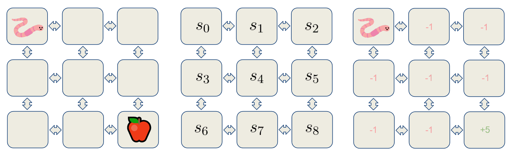
Let’s examine an example of a learnable environment in which a worm is trying to navigate toward an apple. In this case, the worm will be an agent, and the tiles that he can travel on will signify the states.

Moreover, each state gives out a reward. In this example, the worm will receive a reward of $-1$ for entering every state except the one containing the apple. If it reaches that state, he gets a reward of positive $5$ :

Thus, this is a minimal example of an RL problem. However, the environment is usually quite complex and almost impossible to fully understand. This is why we use Monte Carlo methods to sample the environment and gain some knowledge about it.

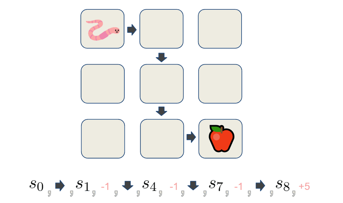
We set out our agent to follow a given policy $\pi$ and interact with the environment until it reaches some terminal state at time $T$ . We term such a traversal as an episode. An episode consists of a sequence of states, actions, and rewards that the agent got on his path. To illustrate, let’s set our agent to act upon some policy and collect an episode:

The goal here is to collect many episodes of traversals through the environment like the one above. These can then be used to iteratively estimate the real state-value function $v_\pi(s)$ and/or action-value function $q_\pi(s, a)$ .

The state-value function assigns a value to each state based on the expected cumulative reward $R$ when starting in $s$ and following $\pi$ . We use it to assess the quality of a given policy.

The state-action value function, on the other hand, expresses the expected cumulative reward $R$ for a given state $s$ and action $a$ and following $\pi$ . Hence, it’s used to improve the policy. If we have correct estimates of either of these functions, we can say that we’re done with the task, as we can easily construct the optimal policy using their outputs.

3. Exploration vs. Exploitation

The more episodes we collect, the better our estimation of the functions will be. However, there’s a problem. Consider the case when the policy improvement algorithm always updates the policy greedily.

In such a case, the algorithm only takes actions that lead to immediate reward. Moreover, we sample the actions and states that are not on the greedy path. As a result, better rewards will stay hidden from the learning process.

Essentially, we have two choices. First, we can make the best decision given the current information. Alternatively, we can start to explore and find more information. This is also known as the exploration vs. exploitation dilemma.

We look for a middle ground between those. Full-on exploration would require a lot of time to collect the needed information.

On the other hand, full-on exploitation would make the agent stuck into a local reward maximum. There are two approaches to ensure all actions are sampled sufficiently: on-policy and off-policy.

4. On-policy Methods

On-policy methods solve the exploration vs exploitation dilemma by including randomness in the form of a policy. Thus, it selects non-greedy actions with some probability. Moreover, we call them $\epsilon$ -greedy policies as they select random actions with an $\epsilon$ probability. Furthermore, they follow the optimal action with $1-\epsilon$ probability:

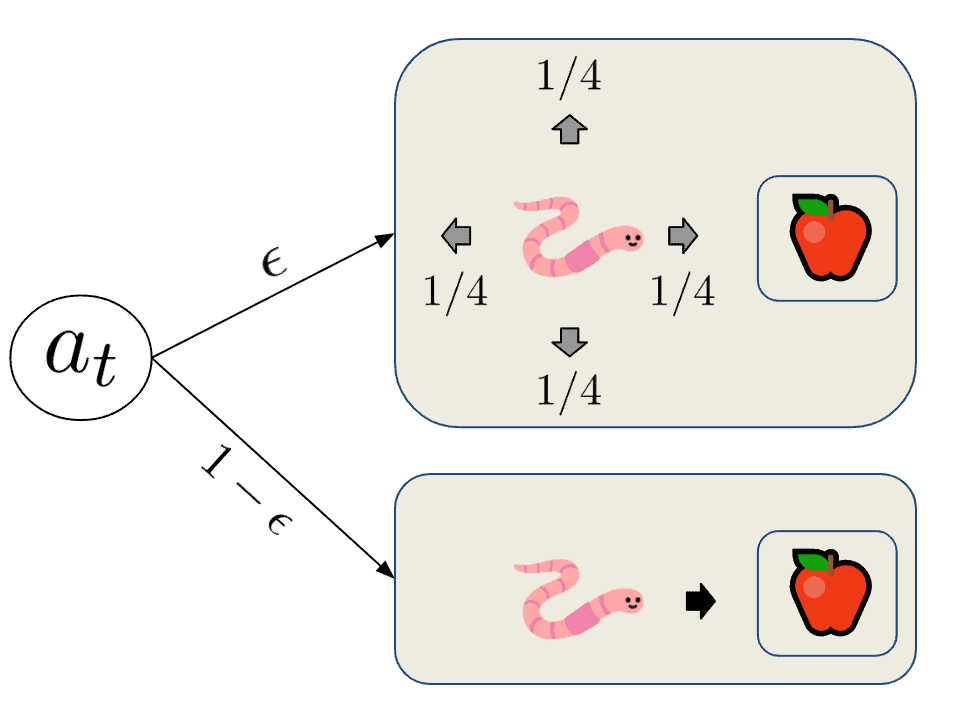
Since the probability of selecting from the action space randomly is $\epsilon$ , the probability of selecting any particular non-optimal action is $\epsilon/|\mathcal{A}(s)|$ . The probability of following the optimal action will always be slightly higher. However, we have a $1 - \epsilon$ probability of selecting it outright and $\epsilon/|\mathcal{A}(s)|∣$ probability of selecting it from sampling the action space:

$P(a_t^{*}) = 1 - \epsilon+\epsilon/|\mathcal{A}(s)|$

Here, it’s also worth noting that we sample the optimal actions more often than the others. Therefore, on-policy algorithms generally converge faster. However, they also have the risk of trapping the agent into a local optimum of the function.

4.1. SARSA

One representative of an on-policy algorithm that uses $\epsilon$ -greedy strategy is state–action–reward–state–action (SARSA). It’s called that way because we’re not using the whole episode to estimate the action-value function $Q$ , but the samples ${S_t, A_t, R_{t+1}, S_{t+1}, A_{t+1}}$ from two subsequent time steps:

$Q^{new}\left(S_{t}, A_{t}\right) \leftarrow Q\left(S_{t}, A_{t}\right)+\alpha\left(R_{t+1}+\gamma Q\left(S_{t+1}, A_{t+1}\right)-Q\left(S_{t}, A_{t}\right)\right)$

Here, $Q^{new}\left(S_{t}, A_{t}\right)$ represents the new $Q$ value. Moreover, $S_t$ and $A_t$ represent the current state and action applied in the current state. Furthermore, $R_{t+1}$ denotes the rewards received by the agent after transiting to the next state $S_{t=1}$ with the action $A_{t+1}$ . Finally, we use $\alpha$ and $\gamma$ to indicate the learning rate and discount factor.

For each state in the episode, SARSA chooses the action $a$ using the $\epsilon$ -greedy policy with respect to the action-value function $Q$ . It receives a reward $R_{t+1}$ and makes a transition to the next state $S_{t+1}$ to make another $\epsilon$ -greedy action $A_{t+1}$ .

5. Off-policy Methods

Off-policy methods offer a different solution to the exploration vs. exploitation problem. While on-policy algorithms try to improve the same $\epsilon$ -greedy policy, off-policy approaches have two policies: a behavior policy and a target policy.

We use the behavioral policy $b$ for exploration and episode generation. Here, we utilize the target policy $\pi$ for function estimation and improvement.

This works because the target policy $\pi$ gets a balanced view of the environment. Additionally, it can learn from potential mistakes of $b$ while still keeping track of the good actions and trying to find better ones.

However, one thing to remember is that in Off-policy learning, there is a distribution mismatch between the population we’re trying to estimate and the one we’re sampling from. That is why we use the importance sampling method to facilitate this mismatch.

5.1. Q-Learning

A very popular off-policy learning to consider is SARSA Max, also known as $Q$ -learning. Here, we try to update the Q function not by choosing $\epsilon$ -greedy actions but rather by always choosing the action with the maximum value:

$Q^{new}(S_{t}, A_{t}) \leftarrow (1 - \alpha) Q(S_{t}, A_{t}) + \alpha \left( R_{t+1} \ + \ \gamma \max_{a} Q(S_{t+1}, a)\right)$

We can see that in the formula, we’re updating the function using both $A_t$ , which is chosen by the $\epsilon$ -greedy policy b, and $\max _{a} Q\left(S_{t}, a\right)$ which is selected by the other greedy “max” policy.

6. Conclusion

In this article, we reviewed the basics of reinforcement learning and examined two families of approaches: on-policy and off-policy learning.

Moreover, we used two popular algorithms, SARSA and Q-learning, as examples. We saw how they battled the problem of exploration vs. exploitation and what each approach offers.

Learn Java Collections

Learn Spring

Learn Maven

View All Courses

Core Concepts

Operating Systems

Neural Networks

Graph Theory

Latex

Full Archive

About Baeldung