Learn through the super-clean Baeldung Pro experience:
>> Membership and Baeldung Pro.
No ads, dark-mode and 6 months free of IntelliJ Idea Ultimate to start with.
Last updated: March 24, 2023

Learn through the super-clean Baeldung Pro experience:
>> Membership and Baeldung Pro.
No ads, dark-mode and 6 months free of IntelliJ Idea Ultimate to start with.
We interact with the environment all the time. Every decision we make influences our next ones in some unknown way. This behavior is the core of Reinforcement Learning (RL), where instead the rules of interaction and influence are not unknown, but predefined.
RL algorithms can be either Model-free (MF) or Model-based (MB). If the agent can learn by making predictions about the consequences of its actions, then it is MB. If it can only learn through experience then it is MF.
In this tutorial, we’ll consider examples of MF and MB algorithms to clarify their similarities and differences.
In Reinforcement Learning, we have an agent which can take action in an environment. Additionally, there are probabilities associated with transitioning from one environment state to another. These transitions can be deterministic or stochastic.
Ultimately, the goal of RL is for the agent to learn how to navigate the environment to maximize a cumulative reward metric.
Finally, we define the policy as the algorithm the agent refines to maximize reward.
Crucially, it is the policy that can be MF or MB. First, let’s start exploring what an MF policy means!
Put simply, model-free algorithms refine their policy based on the consequences of their actions. Let’s explore it with an example!
Consider this  environment:
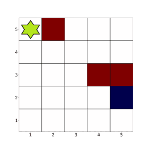
In this example, we want the agent (in green) to avoid the red squares and reach the blue one in as few steps as possible.
To achieve this, we need to define an appropriate reward function. Here’s one way:
The agent has 4 possible actions: left, right, up, and down. On the edges, it has only 2 or 3 of these choices.
Let’s see how Q-learning can be used to optimize the agent’s actions.
Let’s take 15 episodes of 1000 iterations.
Here’s a plot of the agent performance given by average reward per episode:
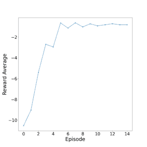
As we can see, the agent learns the task well at around 8 episodes (8000 iterations).
However, Q-learning suffers from being short-sighted with rewards. This can be partially addressed by using Deep Q-learning, which uses a neural network instead of a Q-table.
Nevertheless, Q-learning tends to be faster to compute than model-based methods. This is due to not using a model of the environment.
In a way, we could argue that Q-learning is model-based. After all, we’re building a Q-table, which can be seen as a model of the environment. However, this isn’t how the term model-based is used in the field.
To classify as model-based, the agent must go beyond implementing a model of the environment. That is, the agent needs to make predictions of the possible rewards associated with certain actions.
This provides many benefits. For example, the agent interacts with the environment a few times. Then, the model uses this information to simulate subsequent iterations without needing to interact with the environment.
Using supervised learning, we can optimize the model to determine which trajectories are most likely to generate the biggest rewards.
If done well, this can speed up learning by orders of magnitude.
However, the model uses information provided by the agent, which is finite. Therefore, we run the risk of building a bad model – one that leads to the agent making sub-optimal decisions.
Let’s explore this further.
One model-based algorithm that reduces this risk is Model Predictive Control.
As before, an optimal trajectory is determined. However, only one action is taken by the agent and then a new optimal is determined.
This way, we need fewer optimization steps for the trajectory. If done correctly, this can further speed up the RL algorithm without reducing performance.
Let’s go back to our previous example to illustrate how model-based RL could be useful.
First, let’s assume that the actions are now stochastic. Therefore, a given action has a probability of landing in each neighboring square.
Say the agent finds themselves in this arrangement:
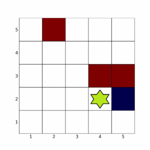
Now, if the actions were deterministic, it’s clear that moving to the right is optimal.
However, in this stochastic example, let’s say that action is highly unlikely to lead to a movement to the right.
A model-based algorithm could approximate these probabilities and then simulate trajectories. It may then inform the agent that, for example, moving down, right, then up is much more likely to produce higher rewards.
An example of such an algorithm is Monte Carlo Learning. It works by collecting agent action trajectories per episode. It then tunes the behavior of the agent based on these sampled trajectories.
Unlike methods like Model Predictive Control, it does not model any trajectories and therefore has no bias. However, the tuning only happens after each episode, which can make the algorithm slow.
In this article, we have built an intuition for the difference between MB and MF RL algorithms. We did this by exploring the basics of RL and using that foundation to explore the differences between the two types of algorithms through a simple example.