

Learn through the super-clean Baeldung Pro experience:
>> Membership and Baeldung Pro.
No ads, dark-mode and 6 months free of IntelliJ Idea Ultimate to start with.
Learn through the super-clean Baeldung Pro experience:
>> Membership and Baeldung Pro.
No ads, dark-mode and 6 months free of IntelliJ Idea Ultimate to start with.
In this tutorial, we are going to discuss the difference between dynamic programming and Q-Learning. Both are classes of algorithms that create a model based on a given environment. They are used to create policies, deciding which actions yield optimal results.
To use a dynamic programming algorithm, we need a finite Markov Decision Process (MDP) to describe our environment. Thus we need to know the probabilities that our actions have. The result we yield is deterministic, e.g., the policy we retrieve with the help of our dynamic programming algorithm is always the same. Another benefit is that it always converges.
Since this is a rather abstract description of how Markov decision process and dynamic programming work, let’s get started with an example.
A simple example of a Markov decision process is to describe the states of a baby. As we can see, the baby can either sleep, be calm, cry or be happy. From the sleeping and the calm state, it is possible to choose between two actions, sing or wait:
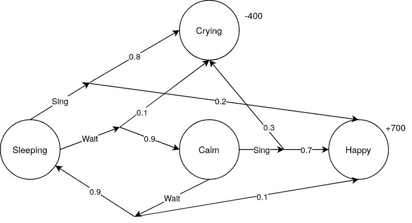
We can see that all the probabilities are given. If we choose an action, we know exactly with which probability we land in which state. Waiting, for example, has a very low chance of yielding happiness and a low chance of crying.
Contrary to that is singing. It results in a high chance of happiness but also involves a higher risk of a crying baby. The result we want to achieve with dynamic programming is to know which decisions result in the highest reward. This means a combination of a high probability that the child becomes happy. But also a low probability that the child starts crying.
Our final policy  will tell us which action to take at which state. To view this in a mathematical sense, we take a look at the value function
  :
:
The value function describes the expected return, starting from state  following policy
  .
.
To solve our MDP, we want to obtain a policy that tells us at which state we should take which action. dynamic programming includes many different algorithms. We choose the value iteration algorithm to solve our MDP. Value Iteration takes our value function  , plugs in a starting value, and iteratively optimizes it.
At this point, we can see an important characteristic of dynamic programming, breaking a problem into smaller parts and solving them separately. That is to say, to find the perfect solution for our MDP, we first find the best policy from calm to happy and then from sleeping to happy. Then, we can combine the solutions to solve the main problem.
In the context of fishing, one faces the challenge of conserving the size of the population while also maximizing the number of harvested fish. For this, our set of actions consists of how many salmon we fish, and our states are the different fishing seasons. We can model this especially well since we know how the population of salmon shrink and grow.
Another use case exists in the area of online marketing. We imagine having an email list of 100000 people and a list of advertising options such as direct offers, product presentations, reoccurring newsletters, etc. Now we want to figure out which brings the customer from the state uninterested to the state buying and satisfied customer. Since we have a lot of data and know when a customer visits your website or buys something, we can easily create a Markov decision problem.
Another advantage of dynamic programming is that it works deterministically, thus always yielding the same results for the same environment. Therefore it is very popular in finance, as it is very regulated.
Contrary to dynamic programming, Q-Learning does not expect a Markov decision process. It can work solely by evaluating which of its actions return a higher reward. While this stands out as a huge advantage since we don’t always have a complete model of our environment, it is not always certain that our model converges in a particular direction.
To make this idea more clear, we have a look at the same example of the happy baby. This time we do not have the probabilities for each action. We don’t even know which actions result in which state:
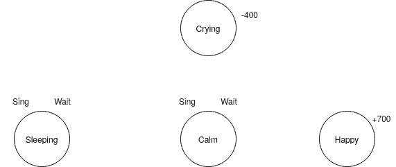
This model might be more realistic. In many real-world cases, we don’t have the probabilities of our action’s outcome.
The principle of Q-Learning is to take future rewards and add a part of those rewards to the steps that came right before them. Thus creating a “path” to the reward, on which we only choose those actions that have a high expected reward. But how do we save those expected rewards and choose the right path?
For this purpose, we make use of the Q-Table. In the Q-Table, we save all our expected rewards in regards to our actions and states. But first, we initialize it with random values. To visualize this further, we have a look at the Q-Table of our example:
| Q-Table | Sing | Wait |
|---|---|---|
| Sleeping | 77 | 71 |
| Calm | 70 | 55 |
| Crying | -400 | -400 |
| Happy | 700 | 700 |
As we already know the expected rewards for crying and happiness for sure, we don’t have to initialize them randomly. Now we evaluate the table. Since singing has the highest value in the first state, we choose singing.
Singing leads us, randomly, to the crying state. Thus we lower the expected reward of sleeping from 77 to 60. The formula to calculate this expected reward is:

 describes the state we are currently in
 describes the action we are taking
 describes the learning rate
 the discount factor
 the expected reward from the next state
This formula describes how the new expected reward is a composition of our old one and a combination of the new value combined with various parameters such as learning rate and discount factor. The learning rate describes how much the new value should override the old one. The discount factor describes how strong far away rewards should affect the current state.
The crying state is a terminating one. That’s why we move on by resetting our environment and starting at our beginning state of sleep again. Now, of course, we choose to wait since the expected reward of waiting, 71, is higher than singing, 60.
We continue this learning process for a fixed number of episodes. How many episodes depend on the context of the environment. Since our example is very small, even 200 episodes are sufficient. For other, more common examples, such as the mountain car environment, we need 25000 episodes of learning or more.
After applying this method, we obtain a q-table that tells us which decision to take in each process:
| Q-Table | Sing | Wait |
|---|---|---|
| Sleeping | -134 | 425 |
| Calm | 590 | -36 |
| Crying | -400 | -400 |
| Happy | 700 | 700 |
We can see that choosing to wait in the sleeping state and choosing to sing in the calm state results in the highest rewards.
To visualize this learning process we have a look at the following flowchart:
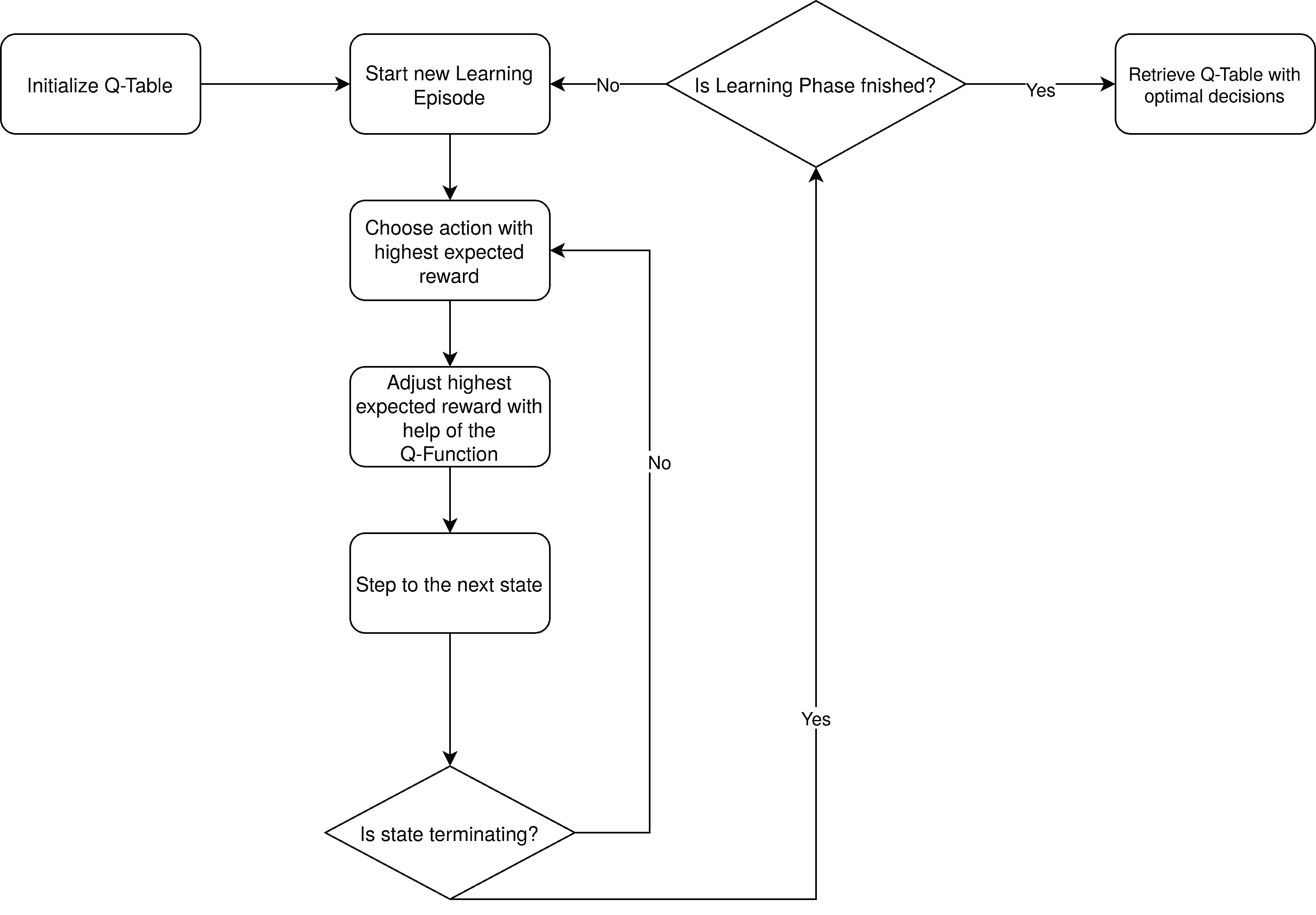
First of all, initialize a Q-Table with random numbers. Then we start our first learning episode, evaluating our expected rewards with the help of our Q-Function  , as stated above.
As soon as we happen to be in a terminating state, we start our next learning episode, as long as the learning phase is not finished yet. If the learning phase is already finished, we retrieve our optimal decision policy from our Q-Table. We simply do this by choosing the cell with the highest value in each row.
In many use cases, we don’t have the probabilities of changing to a particular state given action and a state, and thus reinforcement learning yields better results than dynamic programming. Additionally, the Markov decision process might become extremely big, resulting in resource or time challenges.
The latter is a reason why Q-Learning is a great tool to create Artificial intelligence in games. The biggest example is Alpha Go by google and OpenAI Give from OpenAI. They both managed to beat the worlds leading champions which no algorithm achieved before.
Another application can be found in robotics, where reinforcement learning enables a robot to learn how to walk. Again we do not have the probabilities of the Markov decision process since the physics of this process is incredibly complex.
Dynamic programming creates optimal policies based on an already given model of its environment. Opposed to that is Q-Learning. It creates policies solely based on the rewards it receives by interacting with its environment.
Therefore for a Q-Learning algorithm to work, we only need to know which parameters in our model we want to optimize. Whereas for a DP algorithm to work, you need a deeper understanding of the environment. For both models, we need a set of states, actions, and rewards.
Dynamic programming and Q-Learning are both Reinforcement Learning algorithms. Thus they are developed to maximize a reward in a given environment. In contrast to that are classical machine learning methods, such as SVM or Neural Networks, that have a given set of data and draw conclusions based on them. But there are also combinations of both possible, in the example of Deep Q-Learning.
With deep Q-Learning, we exchange the Q-Table with a neural network because a Q-Table can quickly become very large. Just imagine a state space that contains time or position. This also results in our algorithm not being deterministic anymore.
In this article, we discussed the differences between dynamic programming and Q-Learning.
They both use different models of the environment to create policies for decision-making. On the one hand, we saw that dynamic programming is deterministic. It gives us an optimal solution.
That’s why its strength depends on the strength of the underlying Markov decision process. Reinforcement Learning, on the other hand, works by interacting with its environment and choosing actions that have a high expected reward.
