Epsilon-Greedy Q-learning

1. Introduction

In this tutorial, we’ll learn about epsilon-greedy Q-learning, a well-known reinforcement learning algorithm. We’ll also mention some basic reinforcement learning concepts like temporal difference and off-policy learning on the way. Then we’ll inspect exploration vs. exploitation tradeoff and epsilon-greedy action selection. Finally, we’ll discuss the learning parameters and how to tune them.

2. Q-Learning Algorithm

Reinforcement learning (RL) is a branch of machine learning, where the system learns from the results of actions. In this tutorial, we’ll focus on Q-learning, which is said to be an off-policy temporal difference (TD) control algorithm. It was proposed in 1989 by Watkins.

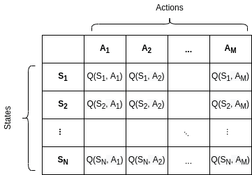
We create and fill a table storing state-action pairs. The table is called $\boldsymbol{Q}$ or Q-table interchangeably.

$Q(S, A)$ in our Q-table corresponds to the state-action pair for state $S$ and action $A$ . $R$ stands for the reward. $t$ denotes the current time step, hence $t+1$ denotes the next one. Alpha ( $\alpha$ ) and gamma ( $\gamma$ ) are learning parameters, which we’ll explain in the following sections.

In this case, possible values of state-action pairs are calculated iteratively by the formula:

$Q(S_t, A_t) \gets Q(S_t, A_t) + \alpha \left[ R_{t+1} + \gamma \max_{a} Q(S_{t+1}, a) - Q(S_t, A_t) \right]$

This is called the action-value function or Q-function. The function approximates the value of selecting a certain action in a certain state. In this case, $Q$ is the action-value function learned by the algorithm. $\boldsymbol{Q}$ approximates the optimal action-value function $\boldsymbol{Q*}$ .

The output of the algorithm is calculated $Q(S, A)$ values. A Q-table for $N$ states and $M$ actions looks like this:

An easy application of Q-learning is pathfinding in a maze, where the possible states and actions are trivial. With Q-learning, we can teach an agent how to move towards a goal and ignore some obstacles on the way.

Let’s assume an even simpler case, where we have the agent in the middle of a 3×3 grid. In this mini example, possible states are the cells of the grid that the agent can reside. Possible actions are (at most) 8 adjacent cells that the agent can travel to. States and action values are:

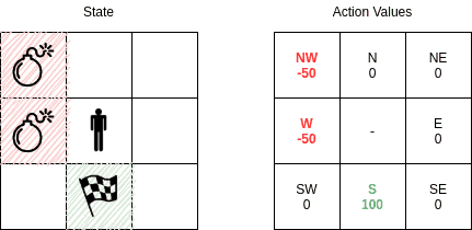
In this case, we can easily represent the Q-values given the state of the agent. In the example above, our state is where the agent is in the middle and has just started. Of course, the agent initially has no idea about its surroundings. As it takes actions, the action values are known to it and the Q-table is updated at each step. After a number of trials, we expect the corresponding Q-table section to converge to:

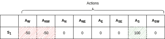
As a result, the agent will ignore the bombs and move towards the goal based on the action values.

3. Q-Learning Properties

Q-learning is an off-policy temporal difference (TD) control algorithm, as we already mentioned. Now let’s inspect the meaning of these properties.

3.1. Model-Free Reinforcement Learning

Q-learning is a model-free algorithm. We can think of model-free algorithms as trial-and-error methods. The agent explores the environment and learns from outcomes of the actions directly, without constructing an internal model or a Markov Decision Process.

In the beginning, the agent knows the possible states and actions in an environment. Then the agent discovers the state transitions and rewards by exploration.

3.2. Temporal Difference

It is a TD algorithm, where the predictions are reevaluated after taking a step. Even incomplete episodes generate input for a TD algorithm. Overall, we measure how the last action is different from what we estimated initially, without waiting for a final outcome.

In Q-learning, Q-values stored in the Q-table are partially updated using an estimate. Hence, there is no need to wait for the final reward and update prior state-action pair values in Q-learning.

3.3. Off-Policy Learning

Q-learning is an off-policy algorithm. It estimates the reward for state-action pairs based on the optimal (greedy) policy, independent of the agent’s actions. An off-policy algorithm approximates the optimal action-value function, independent of the policy. Besides, off-policy algorithms can update the estimated values using made up actions. In this case, the Q-learning algorithm can explore and benefit from actions that did not happen during the learning phase.

As a result, Q-learning is a simple and effective reinforcement learning algorithms. However, due to greedy action selection, the algorithm (usually) selects the next action with the best reward. In this case, the action selection is not performed on a possibly longer and better path, making it a short-sighted learning algorithm.

4. Epsilon-Greedy Q-Learning Algorithm

We’ve already presented how we fill out a Q-table. Let’s have a look at the pseudo-code to better understand how the Q-learning algorithm works:

In the pseudo-code, we initially create a Q-table containing arbitrary values, except the terminal states’. Terminal states’ action values are set to zero.

After the initialization, we proceed by following all the steps of episodes. In each step, we select an action $A$ from our Q-table $Q$ . We’ll talk about epsilon-greedy action selection in the following sections.

As we take action $A$ , our state changes from $S$ to $S'$ . In the meantime, we get a reward of $R$ . Then we use these values to update our Q-table entry $Q(S, A)$ . We repeat until we reach a terminal state.

5. Action Selection

The target of a reinforcement learning algorithm is to teach the agent how to behave under different circumstances. The agent discovers which actions to take during the training process.

5.1. Exploration vs. Exploitation Tradeoff

To better understand how the action selection is performed, we need to first understand the concepts of exploration and exploitation.

In reinforcement learning, the agent tries to discover its environment. As mentioned above, model-free algorithms rely on trial-and-error. During these trials, an agent has a set of actions to select from. Some of the actions are previously selected and the agent might guess the outcome. On the other hand, some actions are never taken before.

In a multi-armed bandit problem, the agent initially has none or limited knowledge about the environment. The agent can choose to explore by selecting an action with an unknown outcome, to get more information about the environment. Or, it can choose to exploit and choose an action based on its prior knowledge of the environment to get a good reward.

The concept of exploiting what the agent already knows versus exploring a random action is called the exploration-exploitation trade-off. When the agent explores, it can improve its current knowledge and gain better rewards in the long run. However, when it exploits, it gets more reward immediately, even if it is a sub-optimal behavior. As the agent can’t do both at the same time, there is a trade-off.

As we already stated, initially the agent doesn’t know the outcomes of possible actions. Hence, sufficient initial exploration is required. If some actions lead to better rewards than others, we want the agent to select these options. However, only exploiting what the agent already knows is a dangerous approach.

For example, a greedy agent can get stuck in a sub-optimal state. Or there might be changes in the environment as time passes. As a result, we wish to keep a balance between exploration and exploitation; not giving up on one or another.

5.2. Epsilon-Greedy Action Selection

In Q-learning, we select an action based on its reward. The agent always chooses the optimal action. Hence, it generates the maximum reward possible for the given state.

In epsilon-greedy action selection, the agent uses both exploitations to take advantage of prior knowledge and exploration to look for new options:

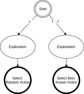
The epsilon-greedy approach selects the action with the highest estimated reward most of the time. The aim is to have a balance between exploration and exploitation. Exploration allows us to have some room for trying new things, sometimes contradicting what we have already learned.

With a small probability of $\boldsymbol{\epsilon}$ , we choose to explore, i.e., not to exploit what we have learned so far. In this case, the action is selected randomly, independent of the action-value estimates.

If we make infinite trials, each action is taken an infinite number of times. Hence, the epsilon-greedy action selection policy discovers the optimal actions for sure.

Now let’s consider the implementation:

As we’ve discussed above, usually the optimal action, i.e., the action with the highest Q-value is selected. Otherwise, the algorithm explores a random action.

An epsilon-greedy algorithm is easy to understand and implement. Yet it’s hard to beat and works as well as more sophisticated algorithms.

We need to keep in mind that using other action selection methods are possible. Depending on the problem at hand, different policies can perform better. For example, the softmax action selection strategy controls the relative levels of exploration and exploitation by mapping values into action probabilities. Here we use the same formula from the softmax activation function, which we use in the final layer of classifier neural networks.

6. Epsilon-Greedy Q-learning Parameters

As we can see from the pseudo-code, the algorithm takes three parameters. Two of them (alpha and gamma) are related to Q-learning. The third one (epsilon) on the other hand is related to epsilon-greedy action selection.

Let’s remember the Q-function used to update Q-values:

$Q(S_t, A_t) \gets Q(S_t, A_t) + \alpha \left[ R_{t+1} + \gamma \max_{a} Q(S_{t+1}, a) - Q(S_t, A_t) \right]$

Now, let’s have a look at the parameters.

6.1. Alpha ( $\boldsymbol{\alpha}$ )

Similar to other machine learning algorithms, alpha ( $\boldsymbol{\alpha}$ ) defines the learning rate or step size. As we can see from the equation above, the new Q-value for the state is calculated by incrementing the old Q-value by alpha multiplied by the selected action’s Q-value.

Alpha is a real number between zero and one ( $0 < \alpha \leq 1$ ). If we set alpha to zero, the agent learns nothing from new actions. Conversely, if we set alpha to 1, the agent completely ignores prior knowledge and only values the most recent information. Higher alpha values make Q-values change faster.

6.2. Gamma ( $\boldsymbol{\gamma}$ )

Gamma ( $\boldsymbol{\gamma}$ ) is the discount factor. In Q-learning, gamma is multiplied by the estimation of the optimal future value. The next reward’s importance is defined by the gamma parameter.

Gamma is a real number between 0 and 1 ( $0 \leq \gamma \leq 1$ ). If we set gamma to zero, the agent completely ignores the future rewards. Such agents only consider current rewards. On the other hand, if we set gamma to 1, the algorithm would look for high rewards in the long term. A high gamma value might prevent conversion: summing up non-discounted rewards leads to having high Q-values.

6.3. Epsilon ( $\boldsymbol{\epsilon}$ )

Epsilon ( $\boldsymbol{\epsilon}$ ) parameter is related to the epsilon-greedy action selection procedure in the Q-learning algorithm. In the action selection step, we select the specific action based on the Q-values we already have. The epsilon parameter introduces randomness into the algorithm, forcing us to try different actions. This helps not getting stuck in a local optimum.

If epsilon is set to 0, we never explore but always exploit the knowledge we already have. On the contrary, having the epsilon set to 1 force the algorithm to always take random actions and never use past knowledge. Usually, epsilon is selected as a small number close to 0.

7. Conclusion

In this article, we’ve discussed epsilon-greedy Q-learning and epsilon-greedy action selection procedure. We learned some reinforcement learning concepts related to Q-learning, namely, temporal difference, off-policy learning, and model-free learning algorithms. Then we’ve discussed the exploration vs. exploitation tradeoff. Lastly, we’ve examined the epsilon-greedy Q-learning algorithm’s hyper-parameters and how to adjust them.

Full Archive

About Baeldung

Core Concepts

Operating Systems

Artificial Intelligence

Graph Theory

Latex