Value Iteration vs. Policy Iteration in Reinforcement Learning

1. Introduction

We can formulate a reinforcement learning problem via a Markov Decision Process (MDP). The essential elements of such a problem are the environment, state, reward, policy, and value.

A policy is a mapping from states to actions. Finding an optimal policy leads to generating the maximum reward. Given an MDP environment, we can use dynamic programming algorithms to compute optimal policies, which lead to the highest possible sum of future rewards at each state.

Dynamic programming algorithms work on the assumption that we have a perfect model of the environment’s MDP. So, we’re able to use a one-step look-ahead approach and compute rewards for all possible actions.

In this tutorial, we’ll discuss how to find an optimal policy for a given MDP. More specifically, we’ll learn about two dynamic programming algorithms: value iteration and policy iteration. Then, we’ll discuss these algorithms’ advantages and disadvantages over each other.

2. Policy Iteration

In policy iteration, we start by choosing an arbitrary policy $\boldsymbol{\pi}$ . Then, we iteratively evaluate and improve the policy until convergence:

We evaluate a policy $\pi(s)$ by calculating the state value function $V(s)$ :

$V(s) = \sum_{s',r'}p(s', r|s,\pi(s))[r+\gamma V(s')]$

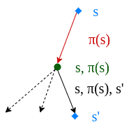
Then, we calculate the improved policy by using one-step look-ahead to replace the initial policy $\pi(s)$ :

$\pi(s) = arg\max_{a} \sum_{s',r'} p(s', r|s,a)[r+\gamma V(s')]$

Here, $r$ is the reward generated by taking the action $a$ , $\gamma$ is a discount factor for future rewards and $p$ is the transition probability.

In the beginning, we don’t care about the initial policy $\pi_0$ being optimal or not. During the execution, we concentrate on improving it on every iteration by repeating policy evaluation and policy improvement steps. Using this algorithm we produce a chain of policies, where each policy is an improvement over the previous one:

$\pi_0 \xrightarrow[]{\text{E}} v_{\pi_0} \xrightarrow[]{\text{I}} \pi_1 \xrightarrow[]{\text{E}} v_{\pi_1} \xrightarrow[]{\text{I}} \pi_2 \xrightarrow[]{\text{E}} \dotsi \xrightarrow[]{\text{I}} \pi_* \xrightarrow[]{\text{E}} v_{*}$

We conduct policy evaluation and policy improvement steps until the policy doesn’t improve anymore:

Since a finite MDP has a finite number of policies, the defined process is finite. In the end, converging an optimal policy $\pi_*$ and an optimal value function $v_*$ is guaranteed.

3. Value Iteration

In value iteration, we compute the optimal state value function by iteratively updating the estimate $\textbf{v(s)}$ :

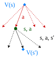
We start with a random value function $V(s)$ . At each step, we update it:

$V(s) = \max_{a} \sum_{s',r'}p(s', r|s,a)[r+\gamma V(s')]$

Hence, we look-ahead one step and go over all possible actions at each iteration to find the maximum:

The update step is very similar to the update step in the policy iteration algorithm. The only difference is that we take the maximum over all possible actions in the value iteration algorithm.

Instead of evaluating and then improving, the value iteration algorithm updates the state value function in a single step. This is possible by calculating all possible rewards by looking ahead.

The value iteration algorithm is guaranteed to converge to the optimal values.

4. Policy Iteration vs. Value Iteration

Policy iteration and value iteration are both dynamic programming algorithms that find an optimal policy $\boldsymbol{\pi_*}$ in a reinforcement learning environment. They both employ variations of Bellman updates and exploit one-step look-ahead:

In policy iteration, we start with a fixed policy. Conversely, in value iteration, we begin by selecting the value function. Then, in both algorithms, we iteratively improve until we reach convergence.

The policy iteration algorithm updates the policy. The value iteration algorithm iterates over the value function instead. Still, both algorithms implicitly update the policy and state value function in each iteration.

In each iteration, the policy iteration function goes through two phases. One phase evaluates the policy, and the other one improves it. The value iteration function covers these two phases by taking a maximum over the utility function for all possible actions.

The value iteration algorithm is straightforward. It combines two phases of the policy iteration into a single update operation. However, the value iteration function runs through all possible actions at once to find the maximum action value. Subsequently, the value iteration algorithm is computationally heavier.

Both algorithms are guaranteed to converge to an optimal policy in the end. Yet, the policy iteration algorithm converges within fewer iterations. As a result, the policy iteration is reported to conclude faster than the value iteration algorithm.

5. Conclusion

We use MDPs to model a reinforcement learning environment. Hence, computing the optimal policy of an MDP leads to maximizing rewards over time. We can utilize dynamic programming algorithms to finding an optimal policy.

In this article, we’ve investigated two algorithms to find an optimal policy for an MDP. Policy iteration and value iteration algorithms work on the same principle. We’ve discussed their advantages and disadvantages over each other.

Full Archive

About Baeldung

1. Introduction

2. Policy Iteration

3. Value Iteration

4. Policy Iteration vs. Value Iteration

5. Conclusion