

Learn through the super-clean Baeldung Pro experience:
>> Membership and Baeldung Pro.
No ads, dark-mode and 6 months free of IntelliJ Idea Ultimate to start with.
Last updated: March 18, 2024
Learn through the super-clean Baeldung Pro experience:
>> Membership and Baeldung Pro.
No ads, dark-mode and 6 months free of IntelliJ Idea Ultimate to start with.
In this article, we’ll introduce one type of neural network that is commonly used in computer vision tasks, called a convolutional neural network (CNN). Besides that, we’ll provide a detailed solution to the problem of constructing this type of network.
There’s a lot of research around this topic and a lot of specific, domain-based CNN architectures are developing. Because of that, there is no one universal answer to the question of how to design this network. Still, there are some useful tips that we can apply in order to upgrade our CNN model and improve predictions of the model.
Neural networks are types of algorithms created as an inspiration for biological neural networks. Initially, the idea was to create an artificial system that would function the way the human brain works. The basis of neural networks are neurons that are interconnected depending on the type of network.
Usually, neural networks consist of layers where each layer consists of multiple neurons. Neural networks that have at least one hidden layer, the layer that is neither input nor output, are called deep neural networks. From that name comes a class of machine learning known as deep learning, where the main focus is deep neural networks.
There are many types of neural networks, but roughly, they fall into three main classes:
The main difference between them is the type of neurons that form them and how the information flows through the network. In this article, we’ll describe only the convolutional class of neural networks.
Convolutional neural networks are a type of artificial neural network, which is a machine learning technique. They’ve been around for a while but have recently gained more exposure because of their success in image recognition. A convolutional neural network is a powerful tool that we can use to process any kind of data where we can apply the convolution operation.
The success of convolutional neural nets is largely attributed to the fact that they can process large amounts of data such as images, videos, and text. Primarily, we can use them to classify images, localize objects, and extract features from the image such as edges or corners. They’re typically composed of one or more hidden layers, each of which contains a set of learnable filters called neurons.
As we’ve mentioned, these networks use convolution that is defined as:
(1) 
where  is the input image and
  is the filter or kernel. More intuitively, we can imagine this process looking at the illustration below:
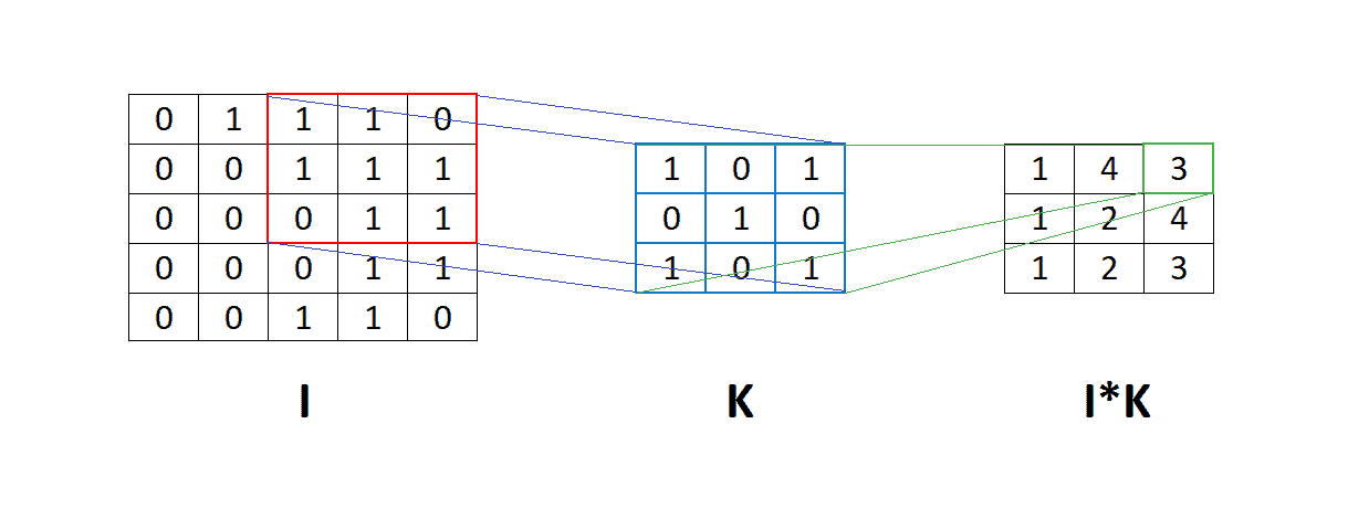
In the image above, we can see the matrix  to which we apply convolution with the filter
  . It means that the filter goes through the whole matrix and element-wise multiplication is applied between the corresponding elements of the matrix and the filter . After that, we sum the result of this element-wise multiplication into one number.
Consequently, the biggest advantage of a convolutional neural network, when compared to a fully connected neural network, is a smaller number of parameters. For example, if the input has  dimension and we apply 10 filters with dimension
  , the output will be a tensor with the format
  . Every filter has
  parameters plus one bias element which is in total for 10 filters
(2) 
parameters. On the other hand, with a fully connected neural network, we would need to flatten the input matrix into a  dimensional vector. In order to have the output with the same dimension as above, we would need
(3) 
parameters, or weights. The weights in the network are what allow it to learn features in different parts of the image. We update these weights through backpropagation, which propagates errors in the output back through the layers to change the weights for training purposes.
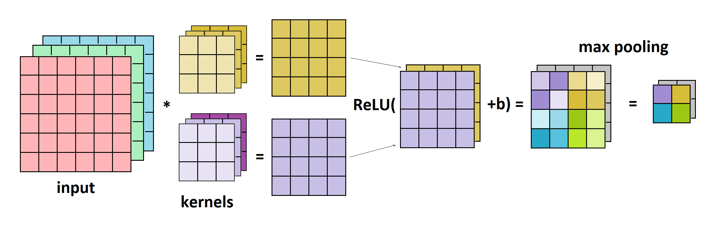
Lastly, it’s worth mentioning that in most cases, the ReLU activation function is being used after the convolutional layer. After that, often follows the pooling layer that applies filters in the same way as the convolutional layer but only calculating the maximal or average item instead of convolution. In the image below, we can see the example of convolutional layer, ReLU, and max pooling:
As we previously mentioned, there is no one generalized rule for creating CNN. It heavily depends on the concrete problem that we are solving. Also, some other factors such as preferable accuracy, training speed, computational resources, and similar might play a significant role in this problem.
For example, for relatively simple problems, such as handwritten digit classification using a popular MNIST data set, we don’t need a complicated CNN architecture. The rule of thumb is to start with a simple CNN that has one hidden layer with around 10 kernels with dimension 3 and one max pooling layer. Based on our results, controlling the trade-off between accuracy and training speed, we can slowly increase the number of kernels and add new layers.
Besides that, we need to keep in mind that the accuracy and speed of the CNN might depend on other factors such as batch size, learning rate, optimizer, and similar. Also, we can try other variations of the ReLU activation function. For instance, Leaky ReLU or ELU functions might provide additional diversification in our neural network.
If we have a more complicated problem, the rule of thumb is to use pre-trained networks. This is possible thanks to a popular technique called transfer learning. It’s a useful and significant method where we can reuse already trained networks despite the fact that they have been trained using different data.
In summary, the process is that we take an already pre-trained model, add one layer or change the last one if necessary, and fine-tune the model using our data set. Transfer learning is possible because the old neural network learned some patterns on the original data set and, with a little tweaking, is able to utilize them in our problem. Of course, the more similar the original data set is to ours, the better results we can expect.
The pre-trained models usually come together with some popular CNN architecture. In most cases, at some point in the past, they achieved state-of-the-art results or were winning solutions for some important competition. We’ll discuss them in more detail next.
One of the most popular and most used data sets in computer vision is ImageNet. It consists of more than 20 million images with almost 22 thousand human-labeled classes. Some of the most popular deep learning packages, including PyTorch, TensorFlow, and others, include pre-trained models trained on this data set. Here, we’ll cover only some of them.
VGG16 is a convolutional neural network that was used in the ImageNet competition in 2014. Number 16 indicates that it has 16 layers with weights, where 13 of them are convolutional and three are dense or fully connected. In addition, it has four max-pooling layers. Examples of VGG16 networks include:
Also known as GoogleNet, InceptionNet is the winner of the ImageNet competition in 2014. This network introduced inception modules that consist of several convolutional layers and one max pooling layer. The idea was to create a good local topology and extract diverse features. In addition, this network used  convolution in order to reduce the channel size in layers. Let’s see a visual representation of an inception module:
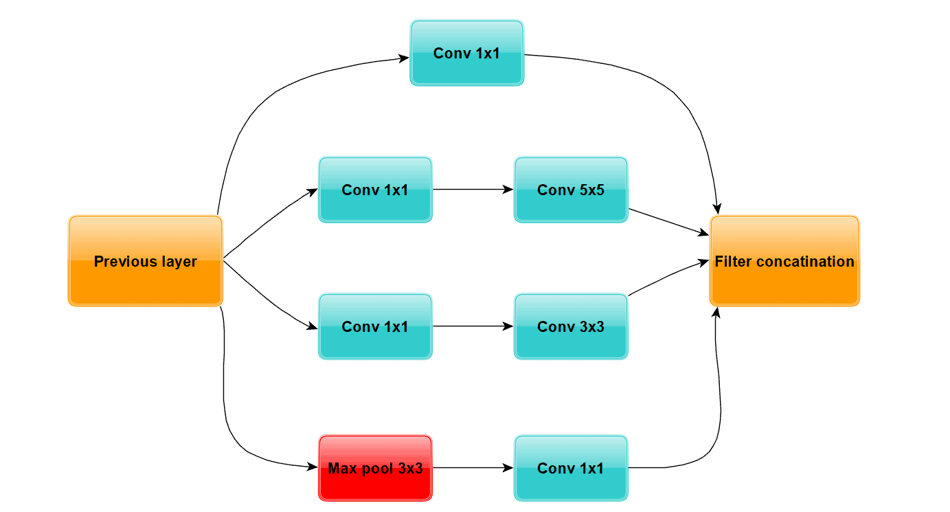
The whole InceptionNet has nine such modules with some other layers. Here are some examples:
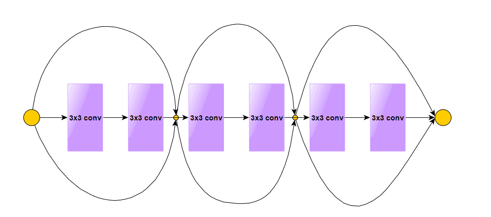
ResNet was the winner of the ImageNet competition in 2015. The authors of this model introduced residual blocks in their network, which was the key to their success. In opposition to traditional neural networks, where each layer feeds into the next layer, some layers in ResNet had a shortcut connection with layers in front. In that way, higher layers were able to get some information from deeper layers directly, and it helped to solve the problem of vanishing gradient.
Let’s see what the residual block looks like:
Similarly, as in previous models, we can find this type of network in PyTorch and TensorFlow as well:
This family of image classifiers was released by DeepMind at the beginning of 2021. and they achieved state-of-the-art accuracy on the ImageNet data set. NFNets (Normalizer-Free Networks) introduce modified residual blocks with scaled weight standardization and adaptive gradient clipping instead of batch normalization. Here’s an example implementation:
Finally, EfficientNets is a family of convolution neural networks, from the smallest  with 5.3 million parameters, up to the biggest
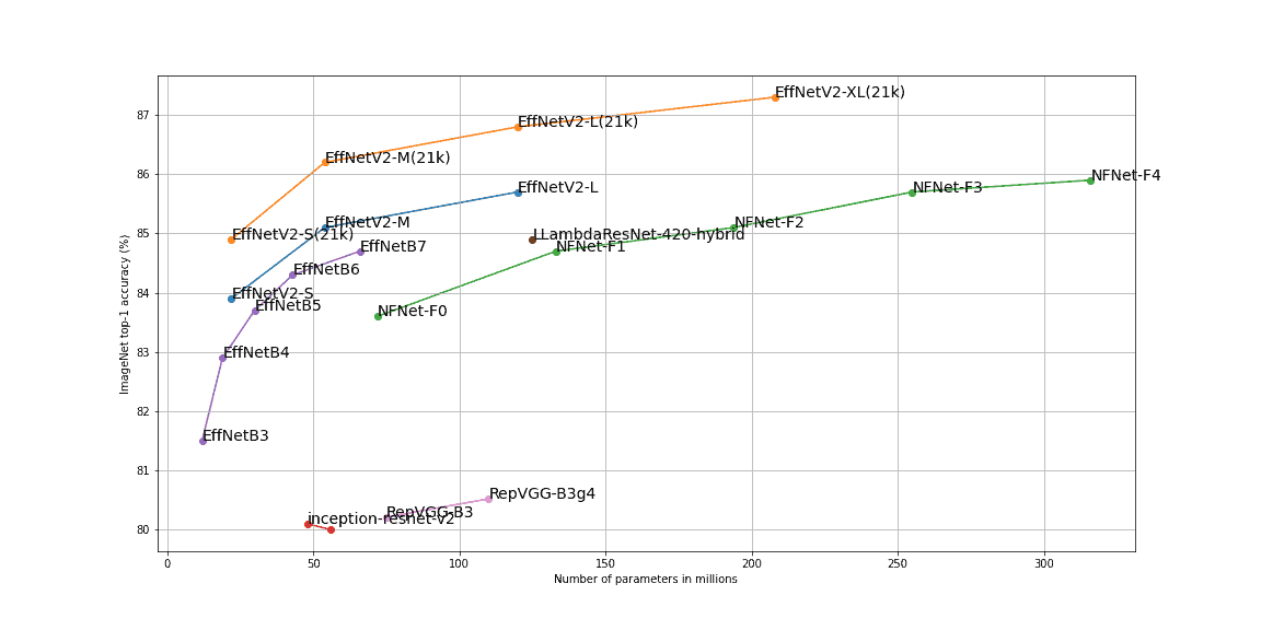
  with 66 million parameters. Although their accuracy had been slightly below NFNet’s accuracy on ImageNet, in late June 2021, Google published a new version, EfficientNetV2, that outperformed all previous CNN architectures.
As a result, this family of networks achieved state-of-the-art results by systematically scaling the depth, width, and resolution of CNN. In addition, V2 uses progressive learning, which means that it progressively increases the sizes of the images through training. Also, they included a new type of layer called the Fused-MB Conv layer. We can see a couple of examples:
Lastly, in the image below, we can see top-1 accuracy on ImageNet of some mentioned networks:
In this article, we’ve studied how to create deep convolutional neural networks. First, we introduced terms of neural networks and convolutional neural networks as well as some basic concepts around them. After that, we described a way of constructing convolution neural networks for both simple and complicated problems. Finally, we showed some of the most used CNN architectures with their state-of-the-art results.