

Yes, we're now running our only Summer Sale. All Courses are 30% off until 20th July, 2026:
Learn through the super-clean Baeldung Pro experience:
>> Membership and Baeldung Pro.
No ads, dark-mode and 6 months free of IntelliJ Idea Ultimate to start with.
1. Introduction
In this tutorial, we’ll study the basic concepts of machine learning and prepare ourselves to approach the study of this fascinating branch of knowledge.
We can consider this article as a small introductory text that explains how the current terminology in machine learning derives from the early studies by the pioneers of the discipline.
We’ll begin by studying the early works by Lovelace and Turing on computing machines. Then, we’ll focus on some key terms that we commonly use today, as they did back then, in the literature by the subject.
2. Background: Can Machines Think?
2.1. Learning Machines
The question that titles this section opens the pivotal paper by Turing, titled Computing Machinery and Intelligence. This question, and the attempts to answer it, are the foundation upon which we built the whole discipline of machine learning.
Both the conceptual system and the terminology that we use today in machine learning derive from Turing‘s initial study on how to potentially answer this particularly deep question; for this reason, it’s a good idea to have a short excursus on it.
Specifically relevant for our purposes is section 7 of that paper, which also concludes it: the section is aptly named “Learning Machines”. It covers the subject of the acquisition of knowledge by computers. In it, Turing responds to Ada Lovelace’s idea that computing machines could only perform actions that they were programmed to do:
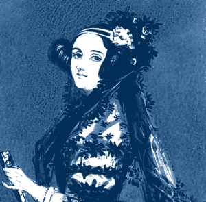
A few years prior, Lady Lovelace had raised the objection, in her study of Babbage’s Analytical Engine, that the capacity by a machine to compute was limited to the instructions that were initially given to it by its programmer. In a sense, she argued, all the ideas that a machine could ever have, are injected into it by a human. They would thus not constitute thinking in the proper sense, in her opinion.
Lovelace was a prominent mathematician of that era and is credited with having developed the first computer algorithms. The theoretical understanding that she had about computation, though, didn’t allow for machines to learn autonomously. All knowledge and learning that could be embedded in a computer, ultimately, was limited by the knowledge and learning that had previously been acquired by that computer’s programmers.
If she had been right, we wouldn’t have a discipline called machine learning today. Clearly, Lovelace’s line of thinking presented some mistakes.
2.2. Learning Humans
Turing argued, in contrast, that the role of the programmers in the learning process would be comparable, at best, to the role that genetics and the initial structure of the brain of a child have on the further development of that child into adulthood. The mind of an adult, according to Turing, was no more determined by the configuration of the brain during childhood, as a computer’s learning capacity was limited by its initial programming.
While the initial configuration of the system certainly played a role in that system’s learning, this wasn’t exhaustive. Two other factors contributed to the learning process of a human. The first was the formal education that a child receives; and the second, the informal experiences to which the child is subject:

As we move from the domain of human learning to the domain of machine learning, the comparison persists. While the initial configuration of given program matters, Turing argued, the learning occurs as a consequence of two additional components. The formal education that the child receives in the computer realm may correspond to the formal training of a model. The informal experiences, instead, correspond to the judgment that the experimenter makes when selecting a certain model over another.
2.3. Learning About Learning
This table sums up the conceptual categories that are common in both human and machine learning, as derived from Turing’s paper:
| Human Learning | Machine Learning |
|---|---|
| Genetics | Initial configuration of the system |
| Formal education | Model training |
| Informal experiences | Evaluation by experimenter |
This is the core of the theoretical basis of the discipline of machine learning and the essence of the deepest problems that it handles:

For each development in the sector of machine learning, human knowledge is advanced, and therefore human learning occurs. But by definition, any developments in the sector of machine learning must make machines learn better or faster: this, in turn, makes it so that the research in machine learning constitutes a non-linear process.
By that same process, humans learn about machines, and machines learn about the world as it is perceived and understood by humans.
3. Basic Concepts of Machine Learning
In the previous section, we learned why it makes sense to consider machine learning as one of the branches of human knowledge. Indeed, it is a branch of knowledge that covers the way in which learning occurs in machines; therefore, as we learn about it, we undertake a human learning process about the machine learning processes. To the extent that machine learning processes are often initiated by humans, we can also state that, as humans learn more about machine learning, machines themselves subsequently learn more.
 Learning machine learning requires knowledge of the basic vocabulary associated with the discipline. Since the discipline falls at the intersection between computer science, statistics, and cognitive sciences, we draw from all these branches of science to derive the subject-specific vocabulary for machine learning.
Here are some of the most important concepts we need to be familiar with.
3.1. Machine
This is the first word that makes up the name of the discipline, and it’s, therefore, the most important. In the broadest sense, a machine is a mechanism that converts some kind of input into some kind of result or behavior and is the subject of the study of mechanics. In computer science, though, with the word machine, we almost always intend a computer or a universal Turing machine.
A universal Turing machine is an abstract machine capable of performing computation. Modern personal computers are, of course, instances of universal Turing machines if we accept the idea that the available memory is significantly larger than the space complexity of our programs.
3.2. Learning
The second word in the name of the discipline arises out of the initial analogy between the process of human learning and the procedures for incrementally building increasingly more accurate statistical models. In more formal terms, and by paraphrasing Mitchell’s definition, learning is a process by which a program executes a task with increasingly better performances by undertaking a particular set of training experiences.
When learning occurs, the error between the predictions of a model and some true labels or values progressively decreases over time. This also leads to the idea that a relationship exists between the learning, or the error in the predictions, and time, such that learning occurs as a function of time.
Since the learning of a machine learning model is frequently divided into the same series of successive steps, it’s also frequent to use “learning” as a synonym for train, test, and validation of a model.
3.3. Model
In machine learning and statistics, a model is a way to describe a system by using mathematical notations and assumptions.
Common categories of models used in machine learning include:
- Regression models, such as linear and logistic regression
- Support vector machines
- Neural networks
The choice of a specific model depends upon the specific task being performed. This makes it valuable to learn not only the theory and the algorithms used in machine learning; but also the heuristics associated with solving any particular tasks.
3.4. Dataset
A dataset is a list of observations related to some characteristics of the social or physical world and generally consists of features and labels. A variety of datasets exist for supervised and unsupervised learning, and their selection for a particular task depends upon the problem we’re studying. A useful reference is the list of datasets curated by the University of California Irvine, which contains the datasets most frequently used by students.
It’s common to subject datasets to a variety of preprocessing steps, such as normalization and splitting, prior to using them for training machine learning models. Whenever a given dataset is too large to be processed in its entirety, as most real-world datasets are, we can feed them in batches to the model that we’re training.
3.5. Prediction and Error or Cost Functions
A specific distinction exists between machine learning models and statistical models. This distinction concerns the necessity that the former have in performing predictions; this isn’t necessarily needed for the latter.
A machine learning model is useful insofar as it makes accurate predictions. For this reason, we usually demand a machine learning model to score well on the accuracy metrics that we employ.
In supervised learning, the prediction can be computed during training. In that case, we generally want to compute the error between the predicted value and some kind of true value or label. When we do that, we can use the difference between the predicted value and the true value in order to determine a cost, which we then use to train the parameters of the model via techniques such as gradient descent.
3.6. Gradient
In simple and intuitive terms, the gradient of a function indicates the direction and steepness of a slope in a function with more than one variable, as calculated according to each of them. For univariate functions, the gradient corresponds to the total derivative:

More generally, the gradient is a vector field associated with a scalar multivariable function that’s differentiable in at least part of its domain. We can indicate with  this function over the variables
  . Then, we can express the gradient
  as a column vector containing the list of partial derivatives
  , for
, for  in
in  :
:

Let’s make a quick example to understand better the concept of the gradient as a vector field and how to calculate it. A simple bivariate trigonometric function  is the sum of two sine waves over two independent variables:

This function has a gradient that we can calculate as the column vector containing the two partial derivatives,  :
:

The value of the gradient at the point  , in this case, would then be:

The gradient, in a sense, generalizes the notion of a derivative. For this reason, we can use it to determine the direction of the closest stationary points in their associated functions. This is useful to minimize or maximize some functions, such as the cost functions that link the parameters and the predictions of a machine learning model.
Our article on gradient descent and gradient ascent is a good reference to learn more about this process.
4. Conclusion
In this article, we studied the basic concepts of machine learning. We also learned the terminology associated with its basic vocabulary.