Neural Network Architecture: Criteria for Choosing the Number and Size of Hidden Layers

1. Overview

In this tutorial, we’ll study methods for determining the number and sizes of the hidden layers in a neural network.

First, we’ll frame this topic in terms of complexity theory. This will let us analyze the subject incrementally, by building up network architectures that become more complex as the problem they tackle increases in complexity.

Then, we’ll distinguish between theoretically-grounded methods and heuristics for determining the number and sizes of hidden layers.

At the end of this tutorial, we’ll know how to determine what network architecture we should use to solve a given task.

2. Neural Networks and Dimensionality

2.1. The Complexity of Problems and Networks

In our articles on the advantages and disadvantages of neural networks, we discussed the idea that neural networks that solve a problem embody in some manner the complexity of that problem. Therefore, as the problem’s complexity increases, the minimal complexity of the neural network that solves it also does.

Intuitively, we can express this idea as follows. First, we indicate with $C(p)$ some complexity measure of the problem $p$ , and with $C(N)$ the same complexity measure for the neural network $N$ . We can then reformulate this statement as:

$\forall{(p_1, p_2)}\ \forall{(N_1, N_2)}: C(p_1) < C(p_2) \to C(N_1) < C(N_2)$

This statement tells us that, if we had some criteria for comparing the complexity between any two problems, we’d be able to put in an ordered relationship the complexity of the neural networks that solve them.

This is a special application for computer science of a more general, well-established belief in complexity and systems theory. As an environment becomes more complex, a cognitive system that’s embedded in it also becomes more complex.

2.2. Complexity and Curse of Dimensionality

One typical measure for complexity in a machine learning model consists of the dimensionality $|\Theta|$ of its parameters $\Theta$ . This is because the computational cost for backpropagation, in particular, non-linear activation functions, increases rapidly even for small increases of $|\Theta|$ .

This leads to a problem that we call the curse of dimensionality for neural networks. Some network architectures, such as convolutional neural networks, specifically tackle this problem by exploiting the linear dependency of the input features. Some others, however, such as neural networks for regression, can’t take advantage of this.

It’s in this context that it is especially important to identify neural networks of minimal complexity. As long as an architecture solves the problem with minimal computational costs, then that’s the one that we should use. In the following sections, we’ll first see the theoretical predictions that we can make about neural network architectures. Then, if theoretical inference fails, we’ll study some heuristics that can push us further.

3. Neural Networks and Problem Complexity

3.1. The Theoretical Gap in the Literature

In this section, we build upon the relationship between the complexity of problems and neural networks that we gave early. We do so by determining the complexity of neural networks in relation to the incremental complexity of their underlying problems. More concretely, we ask ourselves what the most simple problem that a neural network can solve, and then sequentially find classes of more complex problems and associated architectures is.

This section is also dedicated to addressing an open problem in computer science. There’s an important theoretical gap in the literature on deep neural networks, which relates to the unknown reason for their general capacity to solve most classes of problems. In other words, it’s not yet clear why neural networks function as well as they do.

This article can’t solve the problem either, but we can frame it in such a manner that lets us shed some new light on it. And, incidentally, we’ll also understand how to determine the size and number of hidden layers.

3.2. Degenerate Problems, Degenerate Solutions

The simplest problems are degenerate problems of the form of $y = f(x) = x$ , also known as identities. These problems require a corresponding degenerate solution in the form of a neural network that copies the input, unmodified, to the output:

Simpler problems aren’t problems. Further, neural networks require input and output to exist so that they, themselves, also exist. As a consequence, this means that we need to define at least two vectors, however identical.

3.3. Neural Networks for Linear Separation

A more complex problem is one in which the output doesn’t correspond perfectly to the input, but rather to some linear combination of it. For the case of linear regression, this problem corresponds to the identification of a function $y = f(x, \beta) = \beta \cdot x$ . In here, $\beta$ indicates the parameter vector that includes a bias term $\beta_1$ , and $x$ indicates a feature vector $x = \{x_1, x_2, ..., x_{|x|}\}$ where $x_1 = 1$ .

In the case of binary classification, we can say that the output vector can assume one of the two values $y_1$ or $y_2$ , with $y_1 < y_2$ . Consequently, the problem corresponds to the identification of the same function $f(x, \beta)$ that solves the disequation $y_1 \leq f(x, \beta) \wedge y_2\geq f(x, \beta)$ .

A perceptron can solve all problems formulated in this manner:

This means that for linearly separable problems, the correct dimension of a neural network is $|x|$ input nodes and $|y|$ output nodes. If $|x|$ comprises non-linearly independent features, then we can use dimensionality reduction techniques to transform the input into a new vector with linearly independent components. After we do that, then the size of the input should be $|e|$ , where $e$ indicates the eigenvectors of $x$ .

Consequently, this means that if a problem is linearly separable, then the correct number and size of hidden layers is 0.

3.4. Neural Networks for Non-Linear Separation

The next class of problems corresponds to that of non-linearly separable problems. Non-linearly separable problems are problems whose solution isn’t a hyperplane in a vector space with dimensionality $\mathbb{R}^{|x| \times |y|}$ . The most renowned non-linear problem that neural networks can solve, but perceptrons can’t, is the XOR classification problem. A neural network with one hidden layer and two hidden neurons is sufficient for this purpose:

The universal approximation theorem states that, if a problem consists of a continuously differentiable function in $\mathbb{R}^{|x| \times |y|}$ , then a neural network with a single hidden layer can approximate it to an arbitrary degree of precision.

This also means that, if a problem is continuously differentiable, then the correct number of hidden layers is 1. The size of the hidden layer, though, has to be determined through heuristics.

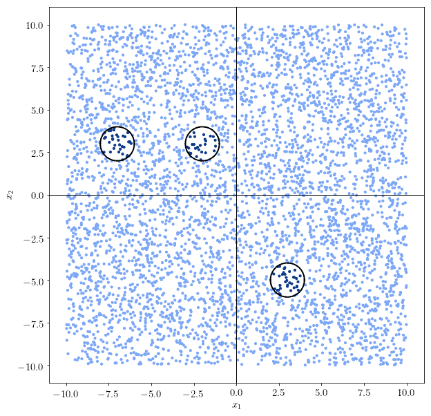
3.5. Neural Networks for Arbitrary Boundaries

The next increment in complexity for the problem and, correspondingly, for the neural network that solves it, consists of the formulation of a problem whose decision boundary is arbitrarily shaped. This is, for instance, the case when the decision boundary comprises of multiple discontiguous regions:

In this case, the hypothesis of continuous differentiability of the decision function is violated. This means that we need to increment the number of hidden layers by 1 to account for the extra complexity of the problem.

Intuitively, we can also argue that each neuron in the second hidden layer learns one of the continuous components of the decision boundary. Subsequently, their interaction with the weight matrix of the output layer comprises the function that combines them into a single boundary.

A neural network with two or more hidden layers properly takes the name of a deep neural network, in contrast with shallow neural networks that comprise of only one hidden layer.

3.6. Neural Networks for Abstraction

Problems can also be characterized by an even higher level of abstraction. With the terminology of neural networks, such problems are those that require learning the patterns over layers, as opposed to patterns over data.

The typical example is the one that relates to the abstraction over features of an image in convolutional neural networks. For example, in CNNs different weight matrices might refer to the different concepts of “line” or “circle”, among the pixels of an image:

The problem of selection among nodes in a layer rather than patterns of the input requires a higher level of abstraction. This, in turn, demands a number of hidden layers higher than 2:

We can thus say that problems with a complexity higher than any of the ones we treated in the previous sections require more than two hidden layers. As a general rule, we should still, however, keep the number of layers small and increase it progressively if a given architecture appears to be insufficient.

3.7. Problems with Even Higher Complexity

Theoretically, there’s no upper limit to the complexity that a problem can have. As a consequence, there’s also no limit to the minimum complexity of a neural network that solves it. On the other hand, we can still predict that, in practice, the number of layers will remain low.

This is because the complexity of problems that humans deal with isn’t exceedingly high. Most practical problems aren’t particularly complex, and even the ones treated in forefront scientific research require networks with a limited number of layers.

For example, some exceedingly complex problems such as object recognition in images can be solved with 8 layers. The generation of human-intelligible texts requires 96 layers instead. This means that, if our model possesses a number of layers higher than that, chances are we’re doing something wrong. To avoid inflating the number of layers, we’ll now discuss heuristics that we can use instead.

4. Heuristics

We can now discuss the heuristics that can accompany the theoretically-grounded reasoning for the identification of the number of hidden layers and their sizes. They’re all based on general principles for the development of machine learning models.

These heuristics act as guidelines that help us identify the correct dimensionality for a neural network. In this sense, they help us perform an informed guess whenever theoretical reasoning alone can’t guide us in any particular problem.

4.1. Build Incrementally More Complex Systems

The first principle consists of the incremental development of more complex models only when simple ones aren’t sufficient. This means that when multiple approaches are possible, we should try the simplest one first. For example, if we know nothing about the shape of a function, we should preliminarily presume that the problem is linear and treat it accordingly. Only if this approach fails, we should then move towards other architectures.

This is because the most computationally-expensive part of developing a neural network consists of the training of its parameters. If we can find a linear model for the solution of a given problem, then this will save us significant computational time and financial resources. If we can’t, then we should try with one or two hidden layers. And only if the latter fails, then we can expand further.

4.2. Prefer Increasing Sizes Over Layers

The second principle applies when a neural network with a given number of hidden layers is incapable of learning a decision function. If we have reason to suspect that the complexity of the problem is appropriate for the number of hidden layers that we added, we should avoid increasing further the number of layers even if the training fails.

Instead, we should expand them by adding more hidden neurons. In fact, doubling the size of a hidden layer is less expensive, in computational terms, than doubling the number of hidden layers. This means that, before incrementing the latter, we should see if larger layers can do the job instead.

Many programmers are comfortable using layer sizes that are included between the input and the output sizes. However, different problems may require more or less hidden neurons than that.

4.3. Process the Data Better

The third principle always applies whenever we’re working with new data. But also, it applies if we tried and fail to train a neural network with two hidden layers. Whenever training fails, this indicates that maybe the data we’re using requires additional processing steps. This, in turn, means that the problem we encounter in training concerns not the number of hidden layers per se, but rather the optimization of the parameters of the existing ones.

Processing the data better may mean different things, according to the specific nature of our problem. For example, maybe we need to conduct a dimensionality reduction to extract strongly independent features. Or perhaps we should perform standardization or normalization of the input, to ease the difficulty of the training. Or maybe we can add a dropout layer, especially if the model overfits on the first batches of data.

Whenever the training of the model fails, we should always ask ourselves how we can perform data processing better. If we can do that, then the extra processing steps are preferable to increasing the number of hidden layers.

5. Conclusion

In this article, we studied methods for identifying the correct size and number of hidden layers in a neural network.

Firstly, we discussed the relationship between problem complexity and neural network complexity.

Secondly, we analyzed some categories of problems in terms of their complexity. We did so starting from degenerate problems and ending up with problems that require abstract reasoning.

Lastly, we discussed the heuristics that we can use. They can guide us into deciding the number and size of hidden layers when the theoretical reasoning fails.

In conclusion, we can say that we should prefer theoretically-grounded reasons for determining the number and size of hidden layers. However, when these aren’t effective, heuristics will suffice too.

Full Archive

About Baeldung

Core Concepts

Operating Systems

Artificial Intelligence

Graph Theory

Latex