Inadequacy of Linear Models: the Road to Nonlinear Functions

1. Introduction

In this tutorial, we’ll analyze the role of activation functions within neural networks. Really, they’ve followed a complex path historically. So, we’ll examine how their epistemological, technical, and mathematical aspects have led us to converge towards nonlinear activation functions.

We’ll begin with linear activation functions and analyze their limitations. We’ll end with some examples that show why using linear activation functions for non-linear problems proves inadequate.

2. Structure of Feed-Forward Neural Networks

We’ll focus our analysis on fully interconnected Feed-Forward Neural Networks, with a structure represented as:

These types of networks have no recursive connections, and each connection connects the units of one layer to all the units of the next layer.

They are an example of supervised neural networks, which learn through the presentation of examples (datasets), comparing the output of the network with the measured value of the relative target.

Propagation occurs from left to right. We’ll denote with the vector $\mathbf{x}$ the set of input units and with $\mathbf{y}$ the set of output units. The unknown relationship that connects inputs and outputs is modeled by the mathematical transformation that occurs within the units.

A deep network is a network containing multiple layers.

2.1. Activation Functions

Next, we want to present the structure of every single unit of the network:

Each connection can amplify or inhibit the value of the relative input $x_i$ through the value of the weight $w_{i}$ . The set of the $N$ connections of each unit is aggregated as a weighted sum:

$\Sigma=w_{0}+\sum_{i=1}^{N}w_{i}x_{i}$

The information mainly resides in the value of the weights. The main purpose of the training process is to find optimal values for the weights.

Bias is considered an additional unit with an output equal to 1 and weight $w_{0}$ . It has the function of $y$ -intercept (offset).

Without bias, the model generated by the network is forced to pass from the origin in the space of the problem, or the point $( \mathbf{x} =0, \mathbf{y} =0 )$ . Bias adds flexibility and allows modeling datasets for which this condition is not met.

The sum $\Sigma$ is transformed according to a function $\phi$ called the activation function. It’s common for the $\phi$ of all units on the network to be the same; however, they can differ. When $\phi$ is nonlinear, then a neural network is capable of modeling a nonlinear relationship present in the data.

An optimal introduction to neural networks is the, already classic, work of Ben Krose and Patrick van der Smag. More technical and deeper treatments are Schmidhuber‘s paper and Bishop‘s book.

3. Knowledge and Models

The main reason for using nonlinear activation functions in artificial neural networks is technical. However, there are also epistemological reasons.

In a sense, the algorithms used in the field of machine learning are the result of an impossibility. This is due to a lack of understanding and knowledge that prevents certain classes of problems from being treated with the traditional scientific approach. The issue is particularly evident in black-box models, such as neural networks.

This fact leads to a change in the operational paradigm and the need to look at these problems from a new point of view. We can express it as the construction of predictive models in ways that imply the renunciation of a deep understanding of the phenomena.

3.1. The Development of Models

In the past three centuries, and until very recent times, knowledge in the empirical sciences has progressed largely through the construction of models. Non-empirical sciences, such as statistics and mathematics in general, have different operating methods.

It’s important to understand that many accepted scientific models and theories are not the result only of the data we measure, but also of qualitative observations of the world.

Let’s think of some very complex physical theories, such as general relativity or quantum mechanics. Today we consider them valid representations of the physical world. But, the road that led to their current formulation has been very long and complex.

Importantly, qualitative knowledge and the possibility of reasoning about the phenomena have allowed us to devise experiments. These experiments led us to compare different options, calibrate the models, and bring them to their current state.

These theories are very accurate in their predictions because this process has allowed us to identify all the variables and parameters on which the physical phenomena depend.

The question is particularly evident when choosing between two theories that can both satisfactorily explain the measured data. In this case, the final choice between the two cannot be made based on their predictive capacity. In this case, they come into play concepts such as generality, simplicity, and elegance.

Occam’s razor, used for centuries in the sciences as a guiding principle, expresses the importance of this type of consideration.

3.2. New Paradigms

The question is that in traditional scientific development certain choices are not true choices. Their linear or nonlinear structure is the result of the theory development process which, as we said, does not depend only on the measured data.

When phenomena are complex, we normally turn to nonlinear models. However, there are many examples of natural laws governed by linear models.

For example, Hook’s law – $F=-kx$ , which connects the force and the displacement of a mass subject to the action of a spring, is an example of a linear model that allows accurate predictions about a real physical phenomenon.

In recent decades, thanks to the ever-increasing calculation capabilities, new needs have arisen. Digital technologies made it possible to collect huge amounts of data, which must be correlated in some way to make predictions.

In these situations, the qualitative component we discussed for physical models is often missing. The reasoning about the world is much more difficult or even impossible and cannot help us in general in the path of identification of the model.

The consequence is that many times, even when a model has been selected, we cannot know if the results obtained are near or far from the best possible solution. This forces us to approach these problems from a new point of view, from a new paradigm.

In these cases, the structure of the model becomes a choice, largely arbitrary, which must be operated with incomplete information.

3.3. An Example

Consider personalized advertising that many online services offer us when we surf the Internet. Their accuracy is essential for advertisers to be interested in promoting their products in this way.

On the surface, we might suppose the ads should depend on age and past purchases. But in what way?

For example, our tastes change over time, so a purchase’s recency probably matters, too. Perhaps we should add the prospect’s geographic area. Are there any other parameters we need?

3.4. The Arbitrariness of the Choice

It’s possible to answer these questions, at least partially.

However, since there’s not even the certainty of having identified all the parameters on which the problem depends, it’s clear that a model built to solve it cannot have the accuracy that we’ve discussed for traditional scientific models.

Neural networks and other black-box algorithms allow building a relationship between the measured data for unknown problems not amenable to analysis in a classical sense. The goodness of these procedures consists of the fact that they allow obtaining a result in finite time, however good or poor. This discussion highlights how the structure of the model underlying an artificial neural network is, to a large extent, an arbitrary choice.

The lack of knowledge about the intrinsic complexity of the problems treated with these algorithms suggests the choice of the most flexible models. The goal is to be in a situation where we are most likely to get good results. These conditions are offered, a priori, by nonlinear models.

4. Linear and Nonlinear Models

Mathematical functions can be classified in many ways, one of which is to divide them into linear and nonlinear.

A linear function is one that satisfies the following general condition:

$f( ax+by ) =af( x ) +bf( y )$

A linear model is, therefore, a procedure governed by linear functions; otherwise, they’re called nonlinear models.

The distinction is important. In a very approximate way, we can consider linear models simpler than nonlinear ones.

In some cases, this distinction gives us an intuition of how the model can evolve as the independent variables and parameters vary, which is much more complicated in the nonlinear models. This is the reason why linear models and equations have historically been studied first.

The complexity of computationally affordable problems nowadays makes it necessary to use nonlinear approaches. However, there are examples of very sophisticated linear procedures. An example is the ARIMA (Auto-Regressive Integrated Moving Average) models, used in the prediction of stationary time series, which make use of linear equations.

Up to now, we’ve implicitly considered that the linearity of the models is given by the linearity of the functions they use. However, we must always consider that a linear statistical model is not the same as a linear function.

A nonlinear function may lead to a linear model. This can happen if linearity is determined by the model parameters and not the predictor variables. We’ll consider the nonlinear character of artificial neural networks as a consequence of the use of nonlinear activation functions.

We can say, in general, that nonlinear models are more flexible and allow us to model more complex phenomena. But, they also have more degrees of freedom and establish more complicated relationships between quantities. So, they’re more difficult to calibrate and test.

4.1. An Intuitive Way of Considering Linear Models

Suppose we want to build a linear model to make predictions about a problem that depends on a single independent variable.

Let’s imagine that we have a series of measurements of a dependent variable – what we’re trying to predict – and of an independent variable. We’ll call the dependent variable our target and the independent variable our input. Then, we can draw these data in a two-dimensional graph.

A linear model consists of the search for the optimal straight line that best explains the measured data. The arrangement of this line on the graph containing the observations gives us a visual idea of the quality of the model.

An example of such a model is the linear least square regression. The goal of this model is to fit a dataset to a straight line that minimizes the deviation of the squares concerning the observations:

pollen raw.dat unsorted normalized train.dat results

To represent a data series of a two-variable problem, we need a three-dimensional graph. In this case, the linear model is constituted by the equation of the plane which best explains the observations.

In general, when the size of the problem grows, the construction of a linear model is formalized as the search for the hyperplane that best adjusts to the observations and allows us to make the most accurate predictions.

When we need to draw a curve to model the problem, then we’re faced with a nonlinear problem.

5. The XOR Problem: A “Simple-Complex” Example

Let’s now take a look at a concrete example. Suppose we have a dataset for which we want to build a model.

As discussed earlier, the structure of the model is arbitrary in a neural network. So, since we don’t want complications, we decide to use a linear model. This attitude assumes that we can obtain acceptable results with both a linear and a nonlinear model.

This claim, however, is false. We’ll demonstrate it with an example.

The XOR operator forms part of the basic bit operators in many programming languages. It can have only two possible values – true or false – and depends on two arguments $( x,y )$ which can also have two possible values.

We can consider it a two-variable mathematical function whose value depends on the truth or falsity of the two propositions or independent variables.

The so-called truth table describes the problem:

x	y	XOR
0	0	0
0	1	1
1	0	1
1	1	0

1	0
0	1

(a)

(b)

The subtable (b) is a way of arranging the truth table as a Cartesian representation.

Unlike the logical disjunction also used in natural language, XOR is false when the two arguments are true. We can consider it a discrete example and analyze it as a classification problem, where the output of the function can belong to two possible categories.

5.1. A Linear Model Cannot Solve XOR

Solving the XOR problem with a linear method means that we can draw a straight line in subtable (b) that perfectly separates the two categories.

However, such a straight line does not exist. In the context of neural networks, a single linear neuron cannot separate the XOR problem, a well-defined and simple problem. This result was formally demonstrated by Minsky and Papert in 1969.

If we use two lines, the problem becomes separable. In a neural network, it means that we have more than one neuron and the network allows obtaining two decision boundaries.

We’ll see in the next section that such an approach cannot be generalized to generic nonlinear problems.

6. Multilayer Network with Linear Activation Functions

The addition of a neuron allows separating the nonlinear XOR problem. This operation increases the number of what we have called “decision boundaries”, and therefore the resolution capacity of the algorithm, which manages to separate the different possibilities.

We can extend this procedure, in principle, to any problem. This implies that we’re able to identify the set of optimal conditions that lead to the linear separability of the problem.

We can think of generalizing this approach, increasing the number of layers and units in each layer, so as to obtain more decision boundaries. However, for highly complex multidimensional nonlinear problems, this approach is not practicable.

XOR is a nonlinear problem, but it can be linearized. This means that we can add additional conditions by dividing our domain into subdomains within each of which the behavior is linear. Mathematically, it means that in each subdomain, the hypothetical mathematical function that governs our problem has a constant derivative, different from other subdomains.

However, a multilayer network with only linear activation functions does not help us in this task.

6.1. Multilayer Neural Networks with Linear Activation Functions

Suppose a network with three layers, $i$ , $j$ , and $k$ . The output of each layer is the input of the next layer, and the overall function expressed by the network is:

$\sum_{i}w_{i}\left(\sum_{j}w_{j}\left(\sum_{k}w_{k}x_{k}+w_{k0}\right)+w_{j0}\right)+w_{i0}$

where each sum extends to all units of each layer and the weights with subindex 0 indicate the bias. With some calculation, this expression boils down to:

$\sum_{i}\sum_{j}\sum_{k}w_{i}w_{j}w_{k}x_{k}+\sum_{i}\sum_{j}w_{i}w_{j}w_{k0}+\sum_{i}w_{i}w_{j0}+w_{i0}$

which corresponds to a network with a single layer $\sum_{k}w'_{k}x_{k}+w'_{0}$ , where:

$w'_{k}=\sum_{j}\sum_{k}w_{i}w_{j}w_{k}$

$w'_{0}=\sum_{i}\sum_{j}w_{i}w_{j}w_{k0}+\sum_{i}w_{i}w_{j0}+w_{i0}$

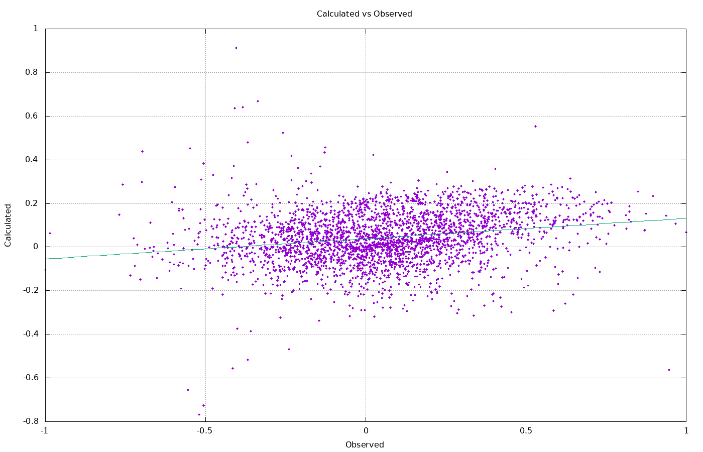
The combination of linear functions is still a linear function, and such a structure can lead to poor results if the relationship existing in the data is intrinsically nonlinear.

It is also possible to demonstrate that the number of units in a one-layer network like this grows exponentially with the size of the problem, being able to arrive at the situation of having an insufficient amount of data to identify all the condition boundaries.

7. Conclusions

In this tutorial, we have made an overview of the differences between linear and nonlinear problems, and how the former are inadequate in dealing with complex nonlinear problems.

The mental approach to problems is essential. For this reason, we briefly also dealt with the question from a methodological point of view. The characteristics of the model underlying an artificial neural network are in part an arbitrary choice, but in general, a linear model is not a good choice.

All these considerations converge to nonlinear activation functions and lead towards nonlinear multilayer networks.

Full Archive

About Baeldung

Core Concepts

Operating Systems

Artificial Intelligence

Graph Theory

Latex