

Learn through the super-clean Baeldung Pro experience:
>> Membership and Baeldung Pro.
No ads, dark-mode and 6 months free of IntelliJ Idea Ultimate to start with.
Learn through the super-clean Baeldung Pro experience:
>> Membership and Baeldung Pro.
No ads, dark-mode and 6 months free of IntelliJ Idea Ultimate to start with.
In this tutorial, we study the theoretical reasons to include bias terms in the architecture of our neural networks.
We’ll first look at some common justifications in favor of bias. Next, we’ll also study some theoretically valid but uncommon justifications for its inclusion in our models.
To do so, we’ll first start by looking at the common-sense meaning of the word bias. This will let us generalize the concept of bias to the bias terms of neural networks.
We’ll then look at the general architecture of single-layer and deep neural networks. In doing so, we’ll demonstrate that if the bias exists, then it’s a unique scalar or vector for each network. This will finally prompt us towards justifying biases in terms of decision surfaces and affine spaces.
At the end of this article, we’ll understand the reasons why bias terms are added to neural networks. But also, and more importantly, we’ll learn exactly where would a neural network without bias have guaranteed prediction errors.
We’re going to first look here at the concept of bias in its general sense. Then, more specifically, we’ll study it in the context of machine learning. The general meaning of bias is, in fact, related to the reason why we include it in the activation functions for neural networks, as we’ll see shortly.
Biases, and their relationship with errors and predictions, are in fact a problem that characterizes not only machine learning, but also the whole discipline of statistical analysis.
In its common meaning, bias is a word that normally indicates a systematic error in the predictions or measurements performed around a certain phenomenon. We say for instance that a person is biased towards an idea if they support it regardless of any contrary evidence. We also say that a game is biased if some players have unfair advantages against the others.
This intuitively tells us that bias is something that happens all the time, regardless of the circumstances of a situation.
In the context of measure theory, bias is related to a so-called true value. True values are epistemological assumptions about what a measurement “would be” if obtained by using an instrument with perfect accuracy. Needless to say, no real-world instruments have perfect accuracy, but the concept still exists.
We can thus imagine that some values for measurements are true, while other legitimately obtained values aren’t. If we do that, we can then note that some instruments systematically report wrong readings against that true value.
If we notice this, we can then recalibrate the instruments to account for this error. In doing so, we can finally obtain only and always true values for measurements.
Interestingly, this process of calibration also occurs in neural synapses and constitutes there what we normally call learning.
If we follow this line of thought, we can thus notice that:
we, therefore, don’t have any errors at all. We would, in that case, simply be left with measurements and the values returned by them.
If we do however have true values, it’s then possible that some specific measurements systematically return errors against them. This systematic error then corresponds to the definition of bias in measurement theory.
Another way to look at this idea is to frame bias as an error in predictions. In that context, the true value is the measurement that we predict to obtain by conducting some observations. In contrast, the bias indicates the degree by which our predictions are off vis-à-vis the empirical observations.
The two definitions of bias as a systematic error in measurements or in predictions are equivalent. The latter however is more suitable in the context of neural networks. Neural networks, in fact, predict values as a function of the input they receive, and we can then study their bias in this framework.
For now, though, we can get familiar with this idea by taking some examples of measurements and predictions in different contexts. While doing this we’ll highlight how some errors can be defined as systematic and subsequently corrected.
We can, for example, imagine performing guesses on the height of some students in a class. Being particularly tall ourselves, we tend to underestimate the height of our students by some 10 centimeters, since from our perspective they all look equally short. In this case, we’d then say that we have a bias towards the idea that individuals are shorter than they really are:
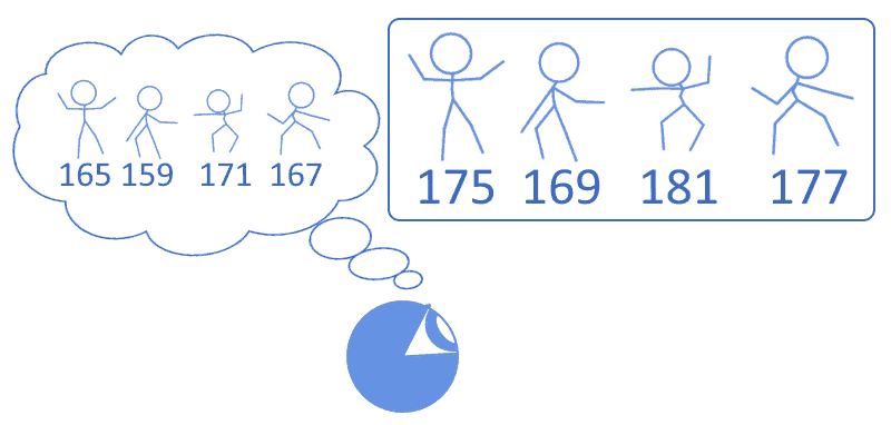
This prejudice can be quantified in the measure of 10 centimeters. Since we know that we hold this prejudice, we can then correct any measurements for it by adding 10 to any specific number that we’d instinctually assign to somebody’s height:
| Our guess | Guess plus error | True value |
|---|---|---|
| 165 | 165+10=175 | 175 |
| 159 | 159+10=169 | 169 |
| 171 | 171+10=181 | 181 |
| 167 | 167+10=177 | 177 |
In this scenario, we’d say that the decision function that we use to assign instinctive values to the students’ heights is biased by 10 centimeters. By adding 10 to any intuitive height that we’d instinctively assign we then could, therefore, compute the true value for that height.
More formally, if  denotes the function through which guess the height of a given student
  , and
, and  is the true height of that student, we can then say that since our predictions are systematically off by 10 centimeters then
  . This way of expressing the problem maps particularly well to the mathematical formulation of bias in neural networks, as we’ll see later.
We can make another example in the context of classification for ordinal categorical variables. The problem of systematic error in measurements, in fact, concerns not only numbers and scalars but also categorical values, and we can treat it analogously for them.
In this second example, we can imagine that the same students as before also possess school degrees, that can assume one of four values:  . Since we, ourselves, didn’t complete middle schools, we have a tendency to overestimate the general level of education of a person:
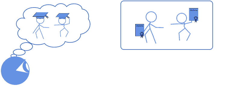
Because we’re aware of our tendency to overestimate this level, we can then correct for our error by shifting all of our instinctive predictions to the precedent degree level:
| Instinctive guess | Shifting by one | True value |
|---|---|---|
| University | College | College |
| College | High School | High School |
| High School | Middle School | Middle School |
In this context, we can say that we held a bias in the assignment of a value to an ordinal categorical variable. In order to correct for this bias, we’ve compensated our instinctual guesses by shifting by a fixed step any spontaneous value that we’d assign to a student’s education.
We can then generalize the considerations made above, in order to formulate a definition of bias in a model and the ways to correct for it, that translates well to neural networks. The examples above show that, if an error is systematically made, we can then take advantage of its predictable nature and compensate for it. As a result, we can still perform accurate predictions as if that error, that bias, didn’t exist at all.
This is regardless of the type of error that’s performed, and in particular regardless of the nature of the variable on which the error is attributed. The keyword here is that the error has to be “systematic”. If this error is systematic, we can then call it “bias” and correct for it in order to obtain true measurements.
The same is valid for predictions. We can state that if our predictions are consistently off by some stable amount  , we can call that amount bias and account for it in our models. The latter is valid whether these models relate to regression or to classification, as we saw earlier, and is generally valid for any task in statistical analysis.
It’s important that we acquire familiarity with the concept of systematic errors because there are known ways to work with them computationally. We’re thus now going to see how to treat biases in neural networks, and will then discuss how to justify their inclusions in the neural networks’ architecture from broader principles of linear algebra and numerical analysis.
We’ll start the discussion on neural networks and their biases by working on single-layer neural networks first, and by then generalizing to deep neural networks.
We know that any given single-layer neural network computes some function  , where
  and
and  are respectively input and output vectors containing independent components. If the neural network has a matrix
  of weights, we can then also rewrite the function above as
  . If both and have dimensionality
  , we can further represent the function
  in a two-dimensional plot:
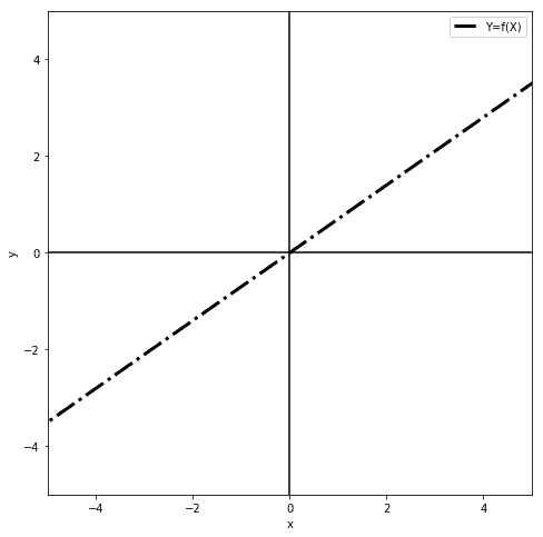
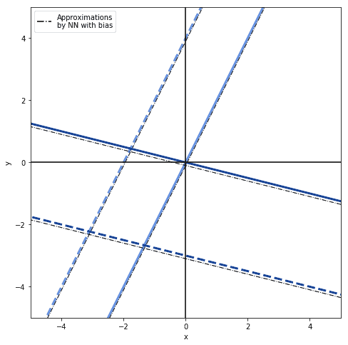
Such a degenerate neural network is exceedingly simple, but can still approximate any linear function of the form  . The function could, but doesn’t have to, indicate a product between and
  such that
  , without including any constant terms. In this case, the neural network can approximate any and all functions passing by the origin but no others:
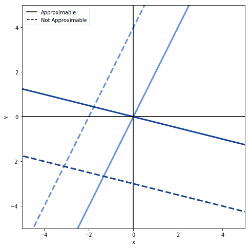
If the function, however, includes a constant term, such that  , then the neural network can approximate any of the linear functions in a plane:
We can start from this intuitive understanding about the behavior of a degenerate neural network and extend it to more complex network architectures.
We can at this point apply the considerations made in the previous section to this toy neural network. If we do that, we can infer that, if there’s any systematic error in the predictions performed by the network, we can call this error and add it to the network’s output to obtain true values.
The calibrated network would then compute a function of the form  . This function would comprise of all the intuitive predictions of the network, to use the terminology of the previous section, simply shifted by the constant . This constant is the bias and it corresponds to that systematic prediction error.
Let’s now add one more input to the network, such that it now computes the function  . Since the two inputs must refer to linearly independent components, we can imagine that
  and
and  both have their own autonomous biases, that we can call
  and
and  .
.
If we do that, we can imagine correcting the predictions of the network by those two independent biases, by computing  . The question now becomes: does this neural network have two biases?
More generally, we’re interested to demonstrate whether the bias in a single-layer neural network is unique or not. We can do this as follows.
First, we repeat the process described above for all independent features ![X = [x_1, x_2, ... , x_n]](/wp-content/ql-cache/quicklatex.com-115e592a1959bafd5c8ff45f841763a8_l3.svg "Rendered by QuickLaTeX.com") and for all of their associated systematic errors
and for all of their associated systematic errors  . If we do so, we can imagine that a single-layer neural network with
  inputs and a weight matrix is actually computing a function
  .
.
Because the linear combination of scalars is also a scalar, we can replace all bias terms associated with each independent input with their linear combination , and rewrite the formula as  . This argument demonstrates that the bias in a layer of a given neural network is a unique scalar. We can now generalize this consideration to neural networks with a number of layers higher than 1.
Let’s now call  the activation function of the layer
  of a neural network with layers, and
  the input to the activation function of layer . We can then say that the neural network is computing the function
  .
.
Let’s also call ![B = [b_1, b_2, ... , b_n]](/wp-content/ql-cache/quicklatex.com-223e7b8069a7dd424363af8110105403_l3.svg "Rendered by QuickLaTeX.com") the vector containing all biases of all layers of the neural network.
the vector containing all biases of all layers of the neural network.  is unique because it’s composed of components that are all unique.
Now, if  and the activation functions
  are odd, as would be the case for the linear unit,
  , or the bipolar sigmoid, the neural network must have a non-null bias vector or it’s guaranteed to diverge from the true values of the dependent variable as approaches zero.
This consideration is particularly important if we use standardized inputs with mean  . In that case, we can expect the neural network to perform poorly if we don’t include a non-zero bias vector.
Unless the network’s activation functions aren’t odd and unless the function which is being approximated isn’t a subspace of the feature space, it’s therefore important to include non-zero bias vectors in the neural network’s architecture.
The situation we described above relates well to some classes of neural networks, such as those that we represent in our tutorial on drawing networks in LaTeX. What if, however, it’s the activation function of each neuron that’s biased, rather than the output of the neuron?
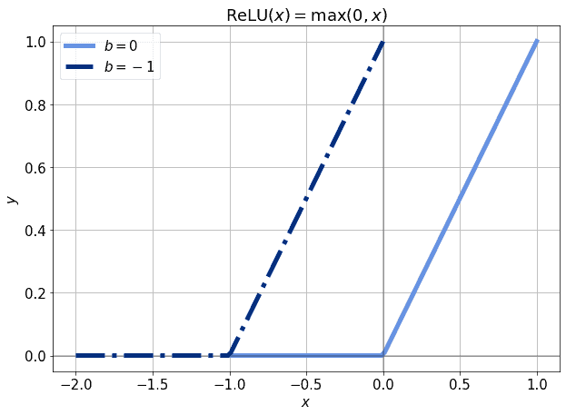
This problem is particularly significant if the activation function that we use is linear or quasi-linear. In that case, in fact, the neurons may frequently end up being inactive, if their input assumes certain values. Consider for example the ReLU function,  :
:

If we’re in the part of the function’s domain for which  , we’re affected by the so-called vanishing gradient problem. However, we could also include a bias term , which acts as an independent input to the ReLU function. This would let us shift the activation function to the left and to the right by simply modifying :
In this manner, even a small value for the bias would be sufficient to initialize the derivatives of the error function to non-zero,  . This would, in turn, allow for backpropagation to happen even when the input is zero. Thus, if we have reason to believe that a certain neuron should be active even when its input is zero, introducing a bias is a good way to do so.
There are proven benefits for introducing a bias term to activation functions for neural networks, regardless of the structure and activation functions. For example, introducing a small bias has been proven to increase performances for Recurrent Neural Networks in a variety of common machine learning tasks. Even if the activation function changes, though, the benefit persists.
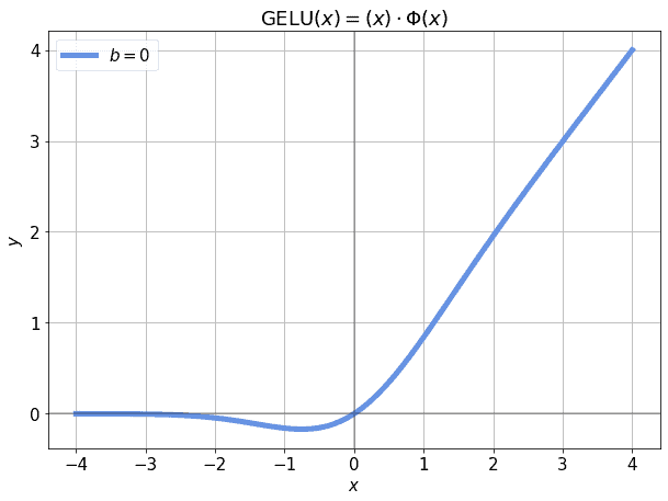
Even more complex forms of the linear unit, such as the recent GeLU which features in BERT, can benefit from a non-zero bias term. For example, if we’ve standardized so that it maps to a normal distribution, we should expect around  of the observations to have a value lower than -3. If that’s the case, the corresponding
  may be very close to zero for those values:
This, in turn, would make the model untrainable with those observations. The incidence of of the observations on a whole dataset isn’t large, of course; however, we’re not justified to use any given observations if we can aprioristically predict that they won’t contribute at all to the training. If, however, we shift the activation function a little, the observations in the neighborhood of -3 will again contribute to the training:
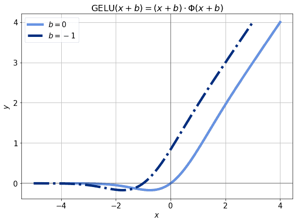
This is because the derivative of the activation function, once again, becomes non-null. As a general rule, adding a bias term to the input of an activation function is, therefore, a good practice, and it justifies well the slight increase in computational time required to train our models.
We can now sum up the consideration made above. This will let us list the conditions which require us to include non-null biases in neural networks. What we’ve seen so far suggests that a neural network needs non-zero bias vectors if:
Let’s now look at this last point in more detail. This will provide us one further justification for the addition of biases in neural networks.
We briefly mentioned in the section above what happens if the target function is a subspace of a network’s space. In that case, we said that we don’t need biases when the activation functions are all odd. Let’s see here why is this the case in terms of decision surfaces of that network.
If the neural network is computing a function of the form , we can then define a vector space  of dimensionality
  where the network operates. Let’s call the vector space of the neural network. The function is then guaranteed to be a subset of but isn’t guaranteed to be a linear subspace.
In order for to be a linear subspace of , it’s necessary for it to include the zero vector. If this happens, then  . That doesn’t guarantee that a function with bias zero is the only one that can approximate
  ; it does however guarantee that at least one such function exists.
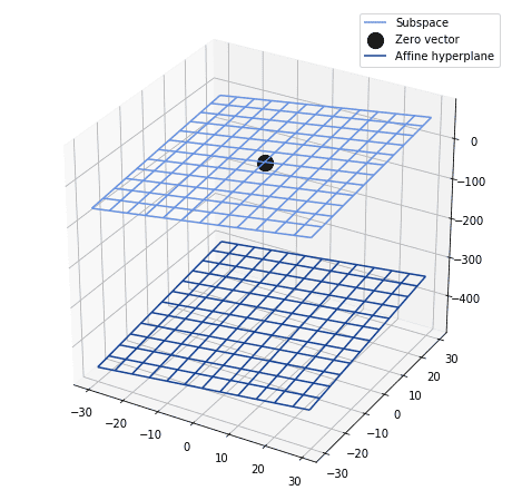
Conversely, it’s also possible that the function corresponds not to a subspace of , but rather to an affine hyperplane of . If this is the case, we then need to include a non-zero bias vector in . Otherwise, the neural network is guaranteed to diverge from the function being approximated as its input tends to zero.
Another way to look at this is to imagine the decision surface of a neural network. We can then ask ourselves what is its relationship with the target function being approximated. This function can consist of either a vector or an affine hyperplane of the vector space for that network. If the function consists of an affine space, rather than a vector space, then a bias vector is required:
If we didn’t include it, all points in that decision surface around zero would be off by some constant. This, in turn, corresponds to a systematic error in that decision that can be rectified by translation.
We could then translate the decision surface by a constant value and call that value bias. In doing so, we’re certain to have a better approximation of the target function in the proximity of zero.
In this article, we studied the formal definition of bias in measurements, predictions, and neural networks. We’ve also seen how to define bias in single-layer and deep neural networks. On the basis of that definition, we’ve demonstrated the uniqueness of a bias vector for a neural network.
We’ve also listed the most common theoretical reasons for the inclusion of biases in neural networks. In addition to this, we also studied a more uncommon argument in their favor under the framework of linear algebra.