

Yes, we're now running our only Summer Sale. All Courses are 30% off until 20th July, 2026:
Introduction to Supervised Learning in Kotlin
Last updated: March 19, 2024
Learn through the super-clean Baeldung Pro experience:
>> Membership and Baeldung Pro.
No ads, dark-mode and 6 months free of IntelliJ Idea Ultimate to start with.
1. Overview
Supervised learning is a subset of machine learning. It consists of training a machine learning model using labeled empirical data. In other words, data gathered from experience.
In this tutorial, we’ll learn to apply supervised learning in Kotlin. We’ll take a look at two algorithms; one simple and one complex. Along the way, we’ll also talk about correct dataset preparation.
2. Algorithms
A supervised learning model is built upon a machine learning algorithm. Multiple kinds of algorithms exist.
Let’s start by looking at some general concepts, and we’ll continue with some of the well-known algorithms thereafter.
2.1. Dataset Preparation
To begin with, we’ll need a dataset. The perfect dataset is prelabeled and its features are relevant and transformed to be given as input to the model.
Unfortunately, the perfect dataset does not exist. Consequently, we’ll need to prepare the data.
Data preparation is crucial when doing supervised learning. Let’s first take a look at our dataset inspired by the Wine Quality Dataset:
| Type | Acidity | Dioxide | pH |
|---|---|---|---|
| red | .27 | 45 | 3 |
| white | .3 | 14 | 3.26 |
| .28 | 47 | 2.98 | |
| white | .18 | 3.22 | |
| red | 16 | 3.17 |
Firstly, let’s begin by handling the missing cells in our dataset. Multiple techniques exist to handle missing data in a dataset.
In our case, for instance, we’ll delete the row containing the missing type of wine because the type is important here as it helps to explain the other features. On the other hand, we’ll also replace the missing numerics by the average of the existing values for the feature:
| Type | Acidity | Dioxide | pH |
|---|---|---|---|
| red | .27 | 45 | 3 |
| white | .3 | 14 | 3.26 |
| white | .18 | 31 | 3.22 |
| red | .26 | 16 | 3.17 |
To clarify, we also made sure to round them up respecting the decimal precision of the column.
Secondly, let’s continue by transforming the categories white and red into numerical values. We consider this feature as being a categorical feature. As for the missing data, multiple techniques apply to categorical data.
In our case, as mentioned earlier, we’ll replace values by numerical values:
| Type | Acidity | Dioxide | pH |
|---|---|---|---|
| 0 | .27 | 45 | 3 |
| 1 | .3 | 14 | 3.26 |
| 1 | .18 | 31 | 3.22 |
| 0 | .26 | 16 | 3.17 |
The last step we’ll take to prepare the dataset will be feature scaling. To clarify, feature scaling is a process to get multiple features on the same scale of values, usually [0, 1] or [-1, 1].
In the case of our dataset, for example, we’ll use min-max scaling.
Min-max scaling is a technique consisting of creating a scale going from the min to the max value of a specific column.
For example, in the Dioxide column, 14 becomes 0 as being the smallest value and 47 will become one. Consequently, all other values will fit in-between:
| Type | Acidity | Dioxide | pH |
|---|---|---|---|
| 0 | .75 | .94 | .07 |
| 1 | 1 | 0 | 1 |
| 1 | 0 | .52 | .86 |
| 0 | .67 | .06 | .68 |
Finally, now that our dataset is prepared, we can focus on the model.
2.2. The Model
The model is the algorithm taking the inputs from our dataset and producing output. In addition, more information on supervised learning algorithms can be found in this introductory article.
Let’s take the example of an artificial neural network to explain the coming concepts with some examples:
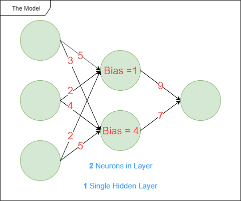
We tend to speak about different kinds of parameters when working on machine learning models. They evolve while the model trains to fit the optimal behavior the model should have. We’ll think about the multiplicators on the input data for example that will be adjusted during training. Some possible parameters are represented by the red values in the illustration.
Other kinds of parameters exist called hyperparameters. Some possible hyperparameters are represented by the blue values in the illustration. These parameters are defined before the training period. Let’s think for instance about the number of neurons needed in an artificial neural network. Another kind of hyperparameter is what kind of activation function to use or what kind of loss function to use.
Let’s now take a look at two kinds of machine learning algorithms: linear regression and artificial neural networks. Other algorithms exist of course (SVM, logistic regression, decision trees or Naive Bayes to name a few) but we’ll not focus on them in this article.
2.3. Linear Regression
Linear regression is, as its name suggests, a regression algorithm. It exists in multiple variants:
- Simple Linear Regression explains one scalar variable by another scalar variable. For example, the price of a house can be explained by the number of square feet
- Multiple Linear Regression also explains one scalar variable. But this time, instead of having one variable as input, we’ll receive multiple ones. In the same case of house pricing prediction, we’ll take into account additional variables like the number of rooms, bathrooms, distance to school and public transportation options.
- Polynomial Linear Regression solves the same problems as the multiple linear regression, but the prediction it will draw is not constantly evolving. The price of housing can rise exponentially for example instead of constantly
- Finally, General Linear Models will explain not one but multiple variables at the same time
Other types of linear regression exist but are less common.
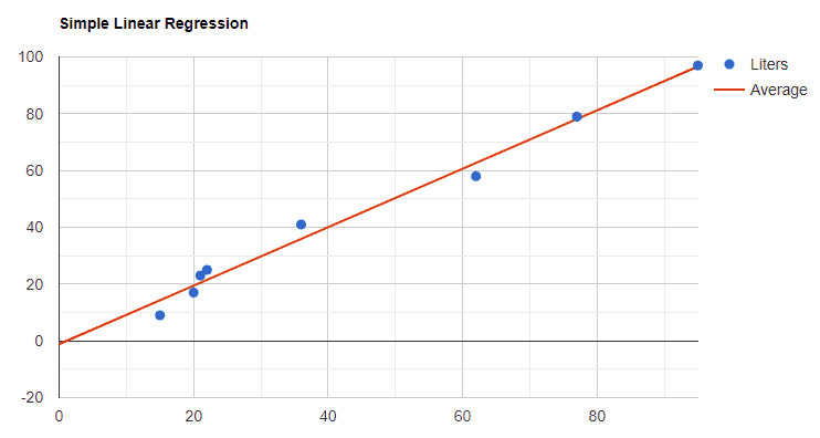
Simply put, linear regression takes a dataset (blue dots) and projects a reasonable line (red) through them for extrapolating conjectures from new data:
2.4. Artificial Neural Networks
Artificial neural networks are more complex machine learning algorithms.
They consist of one or multiple layers of artificial neurons, each layer consisting of one or multiple neurons. Neurons are mathematical functions accepting input and feedforwarding outputs to other neurons or final output.
After the feedforwarding is done, backpropagation is executed to correct the functions’ variables. Backpropagation is needed to lower the cost of the model and by definition increase its accuracy and precision. This is done through the training period using the training dataset.
ANNs can be used to solve regression and classification problems. They usually excel in image recognition, speech recognition, medical diagnosis or machine translation for instance.
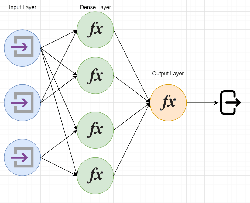
We might visualize an artificial neural network composed of input and output neurons, as well as a hidden layer of neurons (also called a dense layer):
3. Demo Using Native Kotlin
Firstly, we’ll see how it’s possible to create a model natively in Kotlin or any other language. Let’s take simple linear regression for example.
As a reminder, simple linear regression is a model predicting a dependent variable using an independent one. For instance, it could predict the amount of milk necessary in a family depending on the number of children.
3.1. The Formula
Let’s take a look at the formula of simple linear regression and how to get the value of the required variables:
# Variance
variance = sumOf(x => (x - meanX)²)
# Covariance
covariance = sumOf(x, y => (x - meanX) * (y - meanY))
# Slope
slope = coveriance / variance
# Y Intercept
yIntercept = meanY - slope x meanX
# Simple Linear Regression
dependentVariable = slope x independentVariable + yIntercept
3.2. The Formula’s Kotlin Implementation
Let’s now convert this pseudo-code to Kotlin and use a dataset representing the median salary in thousands per year of experience:
// Dataset
val xs = arrayListOf(1, 2, 3, 4, 5, 6, 7, 8, 9, 10)
val ys = arrayListOf(25, 35, 49, 60, 75, 90, 115, 130, 150, 200)
// Variance
val variance = xs.sumByDouble { x -> (x - xs.average()).pow(2) }
// Covariance
val covariance = xs.zip(ys) { x, y -> (x - xs.average()) * (y - ys.average()) }.sum()
// Slope
val slope = covariance / variance
// Y Intercept
val yIntercept = ys.average() - slope * xs.average()
// Simple Linear Regression
val simpleLinearRegression = { independentVariable: Int -> slope * independentVariable + yIntercept }
Now that we have a model built, we can use it to predict values. For instance, how much does someone with 2.5 or 7.5 years of experience should be entitled to earn? Let’s test it:
val twoAndAHalfYearsOfExp = simpleLinearRegression.invoke(2.5) // 38.99
val sevenAndAHalfYearsOfExp = simpleLinearRegression.invoke(7.5) // 128.84
3.3. Evaluating the Result
The result seems to correspond to the expected behavior. But how can we evaluate this statement?
We’ll use a loss function (R² in this case) to calculate how well the years of experience explains the dependent variable salary:
# SST
sst = sumOf(y => (y - meanY)²)
# SSR
ssr = sumOf(y => (y - prediction)²)
# R²
r² = (sst - ssr) / sst
In Kotlin:
// SST
val sst = ys.sumByDouble { y -> (y - ys.average()).pow(2) }
// SSR
val ssr = xs.zip(ys) { x, y -> (y - simpleLinearRegression.invoke(x.toDouble())).pow(2) }.sum()
// R²
val rsquared = (sst - ssr) / sst
Finally, we get 0.95 for R² which means that the years of experience explains with an accuracy of 95% the salary of an employee. This is thus definitely a good model for predictions. Other variables could be negotiation skills or the number of certifications for example to explain the remaining 5%. Or possibly just randomness.
4. Demo Using Deeplearning4j
For the purpose of this demo, we’ll use the Zalando MNIST dataset to train a convolutional neural network. The dataset consists of 28×28 images of shoes, bags and eight other kinds of clothing.
4.1. Maven Dependencies
Firstly, we’ll begin by adding the Deeplearning4j dependency to our simple maven Kotlin project:
<dependency>
    <groupId>org.deeplearning4j</groupId>
    <artifactId>deeplearning4j-core</artifactId>
    <version>1.0.0-beta5</version>
</dependency>
Also, let’s add the nd4j dependency. ND4J provides an API to execute multi-dimensional matrix computations:
<dependency>
    <groupId>org.nd4j</groupId>
    <artifactId>nd4j-native-platform</artifactId>
    <version>1.0.0-beta5</version>
</dependency>
4.2. The Dataset
Now that we’ve added the required dependencies, let’s download and prepare the dataset. It is available from the Zalando MNIST GitHub page. We’ll prepare it by appending the labels at the end of the pixels vectors:
private const val OFFSET_SIZE = 4 //in bytes
private const val NUM_ITEMS_OFFSET = 4
private const val ITEMS_SIZE = 4
private const val ROWS = 28
private const val COLUMNS = 28
private const val IMAGE_OFFSET = 16
private const val IMAGE_SIZE = ROWS * COLUMNS

fun getDataSet(): MutableList<List<String>> {
    val labelsFile = File("train-labels-idx1-ubyte")
    val imagesFile = File("train-images-idx3-ubyte")

    val labelBytes = labelsFile.readBytes()
    val imageBytes = imagesFile.readBytes()

    val byteLabelCount = Arrays.copyOfRange(labelBytes, NUM_ITEMS_OFFSET, NUM_ITEMS_OFFSET + ITEMS_SIZE)
    val numberOfLabels = ByteBuffer.wrap(byteLabelCount).int

    val list = mutableListOf<List<String>>()

    for (i in 0 until numberOfLabels) {
        val label = labelBytes[OFFSET_SIZE + ITEMS_SIZE + i]
        val startBoundary = i * IMAGE_SIZE + IMAGE_OFFSET
        val endBoundary = i * IMAGE_SIZE + IMAGE_OFFSET + IMAGE_SIZE
        val imageData = Arrays.copyOfRange(imageBytes, startBoundary, endBoundary)

        val imageDataList = imageData.iterator()
          .asSequence()
          .asStream().map { b -> b.toString() }
          .collect(Collectors.toList())
        imageDataList.add(label.toString())
        list.add(imageDataList)
    }
    return list
}
4.3. Building the Artificial Neural Network
Let’s now build our neural network. For that, we’ll need:
- multiple convolutional layers – These layers have proven to be optimal in image recognition. Indeed, the fact of working in zones instead of pixel per pixel will allow for better shape recognition
- pooling layers to go along with the convolution layers – Pooling layers are used to aggregate the different pooled values received from the convolutional layers into single cells
- multiple batch normalization layers to avoid overfitting by normalizing the outputs of different layers, be they convolutional or simple feedforward layers of neurons
- multiple regular feedforward neurons layers bridging the output of the last convolutional layer and the neural network model
private fun buildCNN(): MultiLayerNetwork {
    val multiLayerNetwork = MultiLayerNetwork(NeuralNetConfiguration.Builder()
      .seed(123)
      .l2(0.0005)
      .updater(Adam())
      .weightInit(WeightInit.XAVIER)
      .list()
      .layer(0, buildInitialConvolutionLayer())
      .layer(1, buildBatchNormalizationLayer())
      .layer(2, buildPoolingLayer())
      .layer(3, buildConvolutionLayer())
      .layer(4, buildBatchNormalizationLayer())
      .layer(5, buildPoolingLayer())
      .layer(6, buildDenseLayer())
      .layer(7, buildBatchNormalizationLayer())
      .layer(8, buildDenseLayer())
      .layer(9, buildOutputLayer())
      .setInputType(InputType.convolutionalFlat(28, 28, 1))
      .backprop(true)
      .build())
    multiLayerNetwork.init()
    return multiLayerNetwork
}
4.4. Training the Model
We now have a model and dataset ready. We still need a training routine:
private fun learning(cnn: MultiLayerNetwork, trainSet: RecordReaderDataSetIterator) {
    for (i in 0 until 10) {
        cnn.fit(trainSet)
    }
}
4.5. Testing the Model
Moreover, we need a piece of code testing the model against the test dataset:
private fun testing(cnn: MultiLayerNetwork, testSet: RecordReaderDataSetIterator) {
    val evaluation = Evaluation(10)
    while (testSet.hasNext()) {
        val next = testSet.next()
        val output = cnn.output(next.features)
        evaluation.eval(next.labels, output)
    }
    println(evaluation.stats())
    println(evaluation.confusionToString())
}
4.6. Running the Supervised Learning
We can finally invoke all these methods one after the other and take a look at the performance of our model:
val dataset = getDataSet()
dataset.shuffle()
val trainDatasetIterator = createDatasetIterator(dataset.subList(0, 50_000))
val testDatasetIterator = createDatasetIterator(dataset.subList(50_000, 60_000))

val cnn = buildCNN()
learning(cnn, trainDatasetIterator)
testing(cnn, testDatasetIterator)
4.7. Result
Finally, after a few minutes of training, we’ll be able to see how our model is doing:
==========================Scores========================================
 # of classes:    10
 Accuracy:        0,8609
 Precision:       0,8604
 Recall:          0,8623
 F1 Score:        0,8608
Precision, recall & F1: macro-averaged (equally weighted avg. of 10 classes)
========================================================================
   Predicted:         0      1      2      3      4      5      6      7      8      9
   Actual:
0  0          |     855      3     15     33      7      0     60      0      8      0
1  1          |       3    934      2     32      2      0      5      0      2      0
2  2          |      16      2    805      8     92      1     59      0      7      0
3  3          |      17     19      4    936     38      0     32      0      1      0
4  4          |       5      5     90     35    791      0    109      0      9      0
5  5          |       0      0      0      0      0    971      0     25      0     22
6  6          |     156      8    105     36     83      0    611      0     16      0
7  7          |       0      0      0      0      0     85      0    879      1     23
8  8          |       5      2      1      6      2      5      8      1    889      2
9  9          |       0      0      0      0      0     18      0     60      0    938
5. Conclusion
We’ve seen how to use supervised learning to train a machine learning model using Kotlin. We’ve used Deeplearning4j to help us with complex algorithms. Simple algorithms are even implementable natively without any library.
The code backing this article is available on GitHub. Once you're logged in as a Baeldung Pro Member, start learning and coding on the project.