

Learn through the super-clean Baeldung Pro experience:
>> Membership and Baeldung Pro.
No ads, dark-mode and 6 months free of IntelliJ Idea Ultimate to start with.
Last updated: August 30, 2024
Learn through the super-clean Baeldung Pro experience:
>> Membership and Baeldung Pro.
No ads, dark-mode and 6 months free of IntelliJ Idea Ultimate to start with.
In this article, we’ll see the primary advantages and disadvantages of using neural networks for machine learning tasks. At the end of this article, we’ll know when it’s advisable to use neural networks to solve our problems and under what circumstances. We’ll also know, which is equally important, when we should avoid using neural networks and favor other techniques instead.
The types of neural networks we discuss here are feedforward single-layer and deep neural networks. These types of networks were initially developed to solve problems for which linear regression methods failed. At the time in which the ancestor of the neural networks – the so-called perceptron – was being developed, regression models already existed and allowed the extraction of linear relationships between variables.
The problem of representation of non-linear relationships was not generally solvable. The multilayer perceptrons, which we today call neural networks, then entered the scene and presented a solution:
 Feedforward neural networks are networks of nodes that pass a linear combination of their inputs from one layer to another. As they do this, the nodes decide how to modify their inputs, utilizing a given activation function. The activation function of a neuron is the key here. By selecting non-linear activation functions, such as the logistic function
  shown below, the neural network can embed non-linearity in its operation:
 While linear regression can learn the representation of linear problems, neural networks with non-linear activation functions are required for non-linear classes of problems. The first advantage of neural networks is, therefore, their flexibility in addressing problems with non-linear shapes:
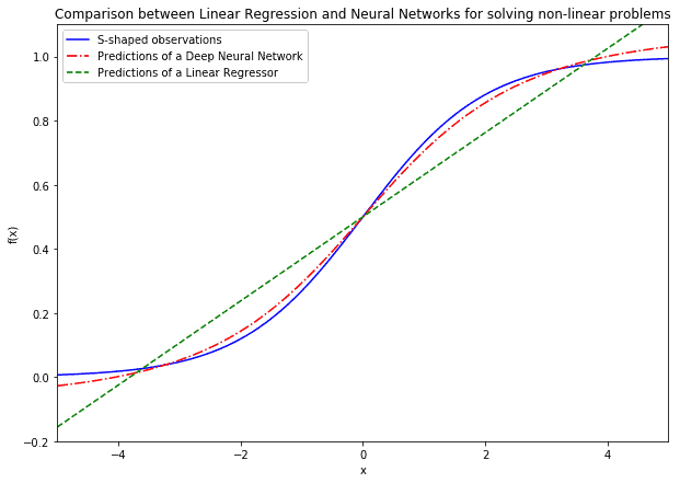 This means that neural networks can generally be tested against a problem with an unknown shape even if other classes of machine learning algorithms have already failed.
The second advantage of neural networks relates to their capacity to approximate unknown functions. The foundational theorem for neural networks states that a sufficiently large neural network with one hidden layer can approximate any continuously differentiable functions. If we know that a problem can be modeled using a continuous function, it may then make sense to use a neural network to tackle it.
A function is continuous if its inputs and outputs are continuous variables, and if the function itself is well defined for all values of its domain. A function is continuously differentiable if its derivative is defined and has one and only one value in all of that function’s domain:
 If the function we study satisfies the condition of continuous differentiability, then neural networks can approximate it by essentially computing its Taylor expansion. However, while it’s proven that neural networks can approximate any continuously differentiable functions, there’s no guarantee that a specific network can ever learn this approximation.
Given a particular initialization of the weights, it may be impossible to learn that approximation using minimization of the loss function and backpropagation of the error. The network may end up stuck in a local minimum, and it may never be able to increase its accuracy over a certain threshold. This leads to a significant disadvantage of neural networks: they are sensitive to the initial randomization of their weight matrices.
Another critical theorem in machine learning states that any given algorithm can solve some classes of problems well but can’t solve some other classes at all. This means that, for any given problem, a specific neural network architecture could be effective, while another will not function well, if at all. Let’s see what this means by comparing perceptrons and deep neural networks against the same problem.
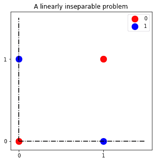
The primary type of problem that neural networks are specifically good at solving is the so-called linearly inseparable problem. The first neural networks were explicitly developed to tackle one of them, given the failure in that sense by their perceptron relatives. This problem was the learning of the XOR function for binary variables, whose graphical representation is:
 Neural networks can learn a separation hyperplane for the classification of the red and blue observations, while perceptrons cannot. One such hyperplane is the one we can see in the figure:
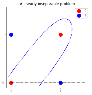 Another way to look at this idea is that if we can’t project the problem onto a hyperplane in which the solution is linearly separable, then perceptrons, themselves one degenerate kind of neural network, will not solve it. At the same time, deep neural networks, another type of neural network, will be able to solve it.
This is a specific case for a more general rule. If one machine learning algorithm is effective at solving one class of problems, it will be ineffective at solving all others. The way around this is to, therefore, have a good theoretical understanding of machine learning in general, and knowledge of the heuristics associated with the resolution of any given task in particular.
Neural networks require for their training, in comparison with other machine learning algorithms, significantly large datasets. They also need significant computational power to be trained. The famous CNN AlexNet for image classification, for example, required six days to train on two GPUs.
A problem then arises when either the dataset or the size of the neural network becomes too large. Neural networks do not generally scale well as the amount of data or the number of their layers and neurons increases. There are several factors that cause this behavior:
We can finally mention that neural networks are typically black box systems. While they can learn abstract representations of a dataset, these representations are hard to interpret by human analysts. This means that while neural networks can, in principle, perform accurate predictions, it’s unlikely that we’ll obtain insights on the structure of a dataset through them.
There’s also another major disadvantage in using neural networks. This time, the issue has to do more with the bias of human programmers than strictly with information theory. Machine learning is excessive and unnecessary for many common tasks. This has nothing to do with neural networks in particular, but it’s a general problem that affects the Data Science community and leads to over-usage of neural networks.
An all-too-frequent case of misapplication of neural networks is when we can solve a problem analytically instead. This issue is prevalent in the machine learning industry today, but it’s frequently ignored. It’s thus crucial that we stress it here. Let’s take as an example the following problem:
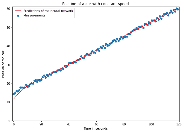
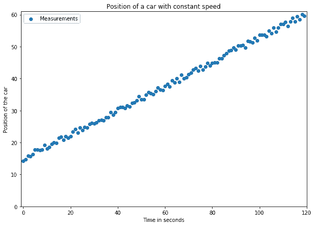 In this problem, a car travels on the street at a constant speed. Our objective is to predict its position at a later time,
  . To do so, we first measure its positions over multiple intervals and obtain the measurements shown in the image above.
The result is a large enough dataset on which we then apply a neural network for linear regression. The dataset in the image above includes errors in the measurements, as per any real-world datasets.
We then divide the dataset into training and testing datasets. On the training dataset, we train a deep neural network, and we measure its accuracy against the testing dataset. After several thousand epochs of training, the network learns that the following relationship exists between the input time  and the output position
  :
:
 This seems like a good result at first glance, but it may not be so if we analyze our work process more thoroughly.
As is common in machine learning tasks, we could measure the accuracy of our system. If we did that, we’d measure very high accuracy and call it a very impressive result. It would also be very trivial, though. Basic domain knowledge in physics would’ve suggested to simply solve the problem analytically. Since the speed is constant, then  and
and  , which we can compute by hand.
Cases such as this one are not uncommon at all in practice, and we should keep them in mind. When tackling a new problem, we shouldn’t try with machine learning straight away. Before doing that, we should look at the literature and see whether an analytical solution is already available. If not, we should first consider developing it ourselves, and only later try working with machine learning.
As a general rule, we should, therefore, not apply neural networks to a problem as a first step. If analytical solutions are unknown, only then should we consider applying simpler machine learning algorithms first, and neural networks second.
In this article, we’ve seen some of the reasons why we should or shouldn’t apply neural networks to our tasks.
Because of the universal approximation theorem, we know that a neural network can approximate any continuously differentiable functions. This is not generally valid for all machine learning algorithms and is a significant advantage of neural networks in particular. We don’t, however, have any guarantees that a neural network can ever learn that approximation.
The No Free Lunch theorem tells us that some network architecture will be the best solution to a given problem. We also know that the same architecture will also be the wrong solution to other problems.
Because of the excessive amount of data and computational power available today, neural networks have become increasingly common. We should use other machine learning algorithms if data or computational power are insufficient.
Some problems allow for analytical solutions that do not require machine learning. In those cases, we should never use neural networks if we can find analytical solutions instead.