

Learn through the super-clean Baeldung Pro experience:
>> Membership and Baeldung Pro.
No ads, dark-mode and 6 months free of IntelliJ Idea Ultimate to start with.
Learn through the super-clean Baeldung Pro experience:
>> Membership and Baeldung Pro.
No ads, dark-mode and 6 months free of IntelliJ Idea Ultimate to start with.
In this tutorial, we’ll study two fundamental components of Convolutional Neural Networks – the Rectified Linear Unit and the Dropout Layer – using a sample network architecture.
By the end, we’ll understand the rationale behind their insertion into a CNN. Additionally, we’ll also know what steps are required to implement them in our own convolutional neural networks.
There are two underlying hypotheses that we must assume when building any neural network:
1 – Linear independence of the input features
2 – Low dimensionality of the input space
The data we typically process with CNNs (audio, image, text, and video) doesn’t usually satisfy either of these hypotheses, and this is exactly why we use CNNs instead of other NN architectures.
In a CNN, by performing convolution and pooling during training, neurons of the hidden layers learn possible abstract representations over their input, which typically decrease its dimensionality.
The network then assumes that these abstract representations, and not the underlying input features, are independent of one another. These abstract representations are normally contained in the hidden layer of a CNN and tend to possess a lower dimensionality than that of the input:

A CNN thus helps solve the so-called “Curse of Dimensionality” problem, which refers to the exponential increase in the amount of computation required to perform a machine-learning task in relation to the unitary increase in the dimensionality of the input.
A trained CNN has hidden layers whose neurons correspond to possible abstract representations over the input features. When confronted with an unseen input, a CNN doesn’t know which among the abstract representations that it has learned will be relevant for that particular input.
For any given neuron in the hidden layer, representing a given learned abstract representation, there are two possible (fuzzy) cases: either that neuron is relevant, or it isn’t.
If the neuron isn’t relevant, this doesn’t necessarily mean that other possible abstract representations are also less likely as a consequence. If we used an activation function whose image includes  , this means that, for certain values of the input to a neuron, that neuron’s output would negatively contribute to the output of the neural network.
This is generally undesirable: as mentioned above, we assume that all learned abstract representations are independent of one another. For CNNs, it’s therefore preferable to use non-negative activation functions.
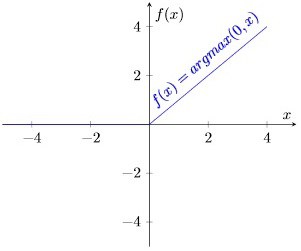
The most common of such functions is the Rectified Linear function, and a neuron that uses it is called Rectified Linear Unit (ReLU),  :
:
This function has two major advantages over sigmoidal functions such as  or
or  .
.
The latter, in particular, has important implications for backpropagation during training. It means in fact that calculating the gradient of a neuron is computationally inexpensive:
<
Non-linear activation functions such as the sigmoidal functions, on the contrary, don’t generally have this characteristic.
As a consequence, the usage of ReLU helps to prevent the exponential growth in the computation required to operate the neural network. If the CNN scales in size, the computational cost of adding extra ReLUs increases linearly.
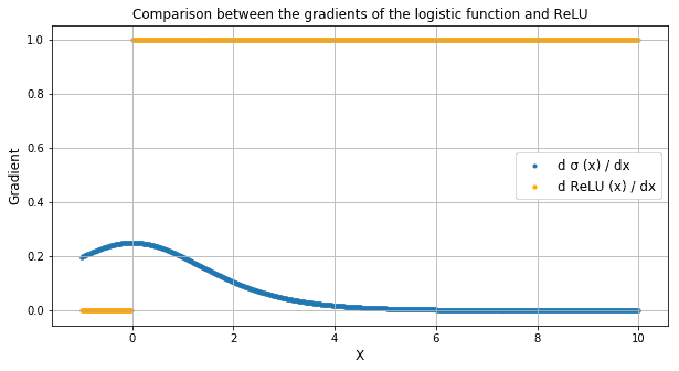
ReLUs also prevent the emergence of the so-called “vanishing gradient” problem, which is common when using sigmoidal functions. This problem refers to the tendency for the gradient of a neuron to approach zero for high values of the input.
While sigmoidal functions have derivatives that tend to 0 as they approach positive infinity, ReLU always remains at a constant 1. This allows backpropagation of the error and learning to continue, even for high values of the input to the activation function:
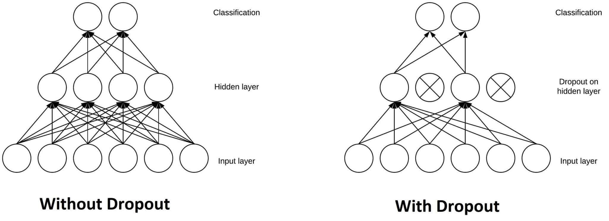
Another typical characteristic of CNNs is a Dropout layer. The Dropout layer is a mask that nullifies the contribution of some neurons towards the next layer and leaves unmodified all others. We can apply a Dropout layer to the input vector, in which case it nullifies some of its features; but we can also apply it to a hidden layer, in which case it nullifies some hidden neurons.
Dropout layers are important in training CNNs because they prevent overfitting on the training data. If they aren’t present, the first batch of training samples influences the learning in a disproportionately high manner. This, in turn, would prevent the learning of features that appear only in later samples or batches:
Say we show ten pictures of a circle, in succession, to a CNN during training. The CNN won’t learn that straight lines exist; as a consequence, it’ll be pretty confused if we later show it a picture of a square. We can prevent these cases by adding Dropout layers to the network’s architecture, in order to prevent overfitting.
This flowchart shows a typical architecture for a CNN with a ReLU and a Dropout layer. This type of architecture is very common for image classification tasks:

In this article, we’ve seen when do we prefer CNNs over NNs. We prefer to use them when the features of the input aren’t independent. We have also seen why we use ReLU as an activation function.
ReLU is simple to compute and has a predictable gradient for the backpropagation of the error.
Finally, we discussed how the Dropout layer prevents overfitting the model during training. Notably, Dropout randomly deactivates some neurons of a layer, thus nullifying their contribution to the output.