

Yes, we're now running our only Summer Sale. All Courses are 30% off until 20th July, 2026:
Learn through the super-clean Baeldung Pro experience:
>> Membership and Baeldung Pro.
No ads, dark-mode and 6 months free of IntelliJ Idea Ultimate to start with.
1. Overview
In this tutorial, we’ll discuss two important conceptual definitions for supervised learning. Specifically, we’ll learn what are features and labels in a dataset, and how to discriminate between them.
We’ll also study the concept of labels for supervised learning tasks and see what is their relationship with our research objectives and our prior knowledge of a phenomenon.
At the end of this tutorial, we’ll know to avoid the common mistake of using labels as if they were features. We’ll also become aware of the prejudices which we include in the machine learning model when we use any given set of labels.
2. Features
Machine learning has its roots in statistical analysis. As a consequence, it’s often very simple to understand concepts in machine learning by looking at their counterpart in statistics.
For example, in statistics, they say that a “population” is a set that statisticians study. In machine learning, instead, we normally called that same full set “a dataset”. Similarly, in statistics, they call each individual in a population a “unit”, while in machine learning we call it “observation”.
The same is valid for features. In statistics, they talk about “variables”, which indicate the characteristics associated with a given statistical unit. In machine learning, we call these characteristics “features”.
We can see that the terminology of the two disciplines is very similar, and it’s often possible to use interchangeably terms from the one or the other.
We can thus say that features are characteristics of observations. Let’s see a few different scenarios in which we try to ascertain the features of observations, to get an intuitive understanding of the concept’s meaning.
2.1. Features as Measurements
One easy way to conceptualize features is to imagine that they are the result of some sensor’s measurements. Let’s imagine we have a thermometer that records the temperature of the air every fifteen minutes. After recording it, it then writes it down on a piece of paper:
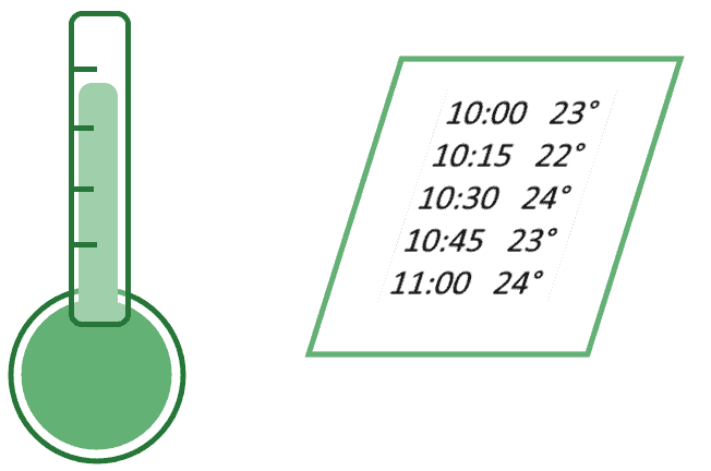
The thermometer performs measurements whose result constitutes a table of observations. The value associated with each measurement corresponds to a feature “temperature”, with machine learning terminology, or a characteristic, in statistical analysis.
Let’s take another example. A police radar measures the speed at which cars go on a street:
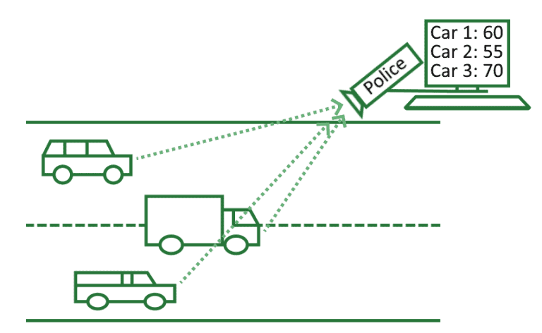
The result is a file in a computer where each row contains the license plate of a vehicle and the speed of that vehicle as measured by the radar.
In this context, the license plates constitute the ID or index of the dataset, and the speed constitutes the features. If we want to learn what cars use a certain street, though, we’re allowed to use the license plates as features, and not just indices.
Let’s take one last example. The spam filter in our email service is monitoring which spam messages are sent between addresses:
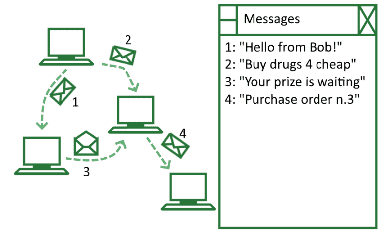
The email server stores a large table containing an index for each email and its associated text. In this case, we can treat the emails as samples or independent statistical units. We can treat instead the texts contained in them as containing the features for a dataset (but see below to learn about texts as features).
The examples we’ve seen show us that we use the term “feature” to reflect the result of an observation or measurement. There are no specific restrictions as to what constitutes a measurement. As a consequence, when approaching a new task, we normally have to spend some time defining it in a manner that allows us to perform measurements in relation to it.
2.2. Types of Task and Identification of Features
We mentioned briefly when discussing the second example above that we can alternatively treat some measurements as either indices or features. Let’s get back to this point and see it in more detail.
When we were talking about the example of the police radar and car speeds, we stated that we might alternatively use the license plates as indices or features of observations. What is the reason why we would do one and not the other in a given concrete situation?
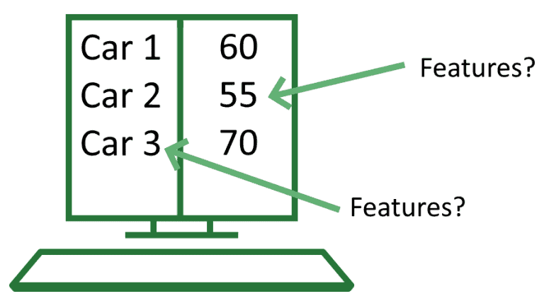
The rationale behind that decision is that it ultimately depends on our objective. Since nobody approaches a problem without background knowledge and expectations about that problem’s characteristics, we can say that our expectations shape our measurements. These expectations, in turn, lead us to identify some of the data collected as “features”, and some of it as indices or noise.
In science, it’s said that measurements are never naive, but are always “theory-laden“. There’s a belief in the machine learning community that it’s possible to conduct measurements and choose features aprioristically and without any expectations on the measurements’ outcome. This is however debated, and potentially capable to blind us to the awareness that our selection of features always implies a prejudice.
This argument supports the idea that we’re free to select whatever features we want when performing measurements. The choice of what data constitutes features and what doesn’t is ultimately in our hands.
2.3. Classes of Features
There are however some common heuristics regarding the selection of features that we can follow to orient ourselves. One of these involves the identification of the class of features that are suitable for a given task. In fact, not all classes of features can be used for all tasks, as we’ll see shortly.
Features can come in a variety of types or classes, that changes slightly from one platform or language to another. The most common types of data for general programming languages are all valid classes for features. These are:
- Integers, floats, and other computable approximations of real numbers
- Preprocessed strings of text, such as “hello world”
- Categories, which we further divide into nominal and ordinal categories
Let’s see them in more detail.
2.4. Approximation of Real Numbers
The most common feature in machine learning datasets consists of integers, floats, doubles, or other primitive data types which approximate real numbers. These are the results of quantitative measurements that we perform with a given instrument.
Numerical data types are the most frequent features used in machine learning. As a consequence, most machine learning techniques can be applied to them.
One of these techniques is for example linear regression. We can perform linear regression by using a numerical feature to predict the value of a target variable:
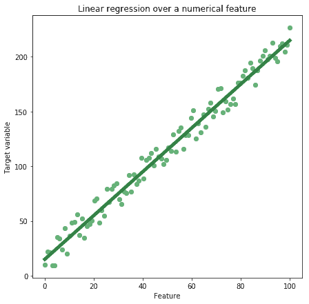
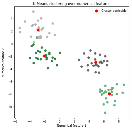
We’ll see later what exactly a target variable is when we’ll talk about labels. Other techniques that work on numerical data types include unsupervised learning techniques, such as K-Means:
Numerical features are the most intuitive ones with which to work. If a measurement produces a number, and if we don’t need to specify anything else about that measurement, then that feature is a numerical feature.
2.5. Texts as Features?
Another typical feature for machine learning tasks is text, or rather a string object. Strings are the primary feature that is used in the subsector of Natural Language Processing for machine learning.
The way in which we treat texts as features for machine learning applications isn’t as direct as was the case for numerical features. It’s in fact not possible to directly treat texts as features, and at the same time be able to extract something useful from a text corpus. There are two main reasons for this.
The first has to do with combinatorics. We could try to treat each character in a string as a random variable that can assume the value of one of the 26 letters of the alphabet. If we did so, each string of length  could assume one of
  possible values, which would make the search space quickly unmanageable:
| n | Combinations |
|---|---|
| 1 | 26 |
| 2 | 676 |
| 3 | 17576 |
| 4 | 456976 |
| 5 | 11881376 |
| 6 | 308915776 |
| 7 | 8031810176 |
And this argument doesn’t take into consideration blank spaces or other characters. The second reason relates to the information content of texts, which isn’t as high as one might think. To this regard, let’s consider this corpus of texts:
| Corpus |
|---|
| The pen is on the table |
| The pen is by the table |
| The pen is under the table |
If we assume we know that the texts talk about a pen and a table, we can then see how most of their words don’t contain useful information. We could, in fact, describe the same corpus in a more reduced format:
| Corpus – processed |
|---|
| pen, table, on |
| pen, table, by |
| pen, table, under |
This is a specific case for a more general rule: Texts aren’t used as features directly, but only after they undertake some kind of preprocessing. These preprocessing steps normally involve stemming and lemmatization, plus tokenization and vectorization. The preprocessed texts then become features for data mining, but texts in their original form aren’t features.
2.6. Categorical Features
A slightly more challenging concept is that of categorical values or features. The idea behind categories is that we can compartmentalize the world and divide it into classes that are mutually exclusive from one another. We can better understand this idea by seeing how it applies to multiple contexts.
For the first example, let’s imagine we sample the color of apples in a given harvest:
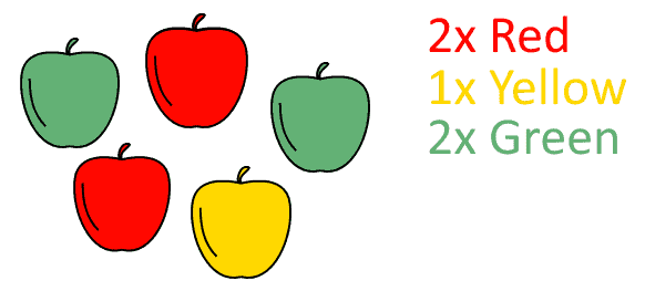
We can safely assume that an apple that’s green isn’t also red, and vice versa, and that the same is valid of all combinations of colors. As a consequence, we can say that the feature “color of the apple” is a categorical feature. Since we have no specific preferential order for them, we can also assume that these categories are unordered.
For the second example, let’s imagine that we’re measuring the level of education in a population:
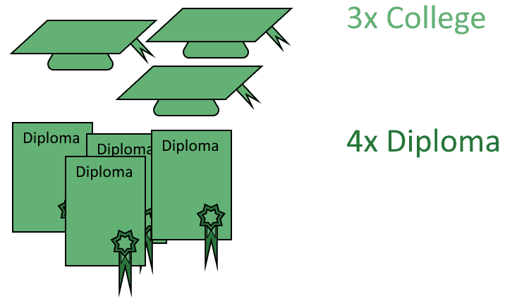
We can safely assume that someone whose highest level degree is a high school diploma doesn’t have a college degree. The opposite is however not true since a person who has a college degree also possesses a diploma.
In this sense, we can establish an order in the distribution of educational degrees. Since college degrees follow diplomas in a student’s life, we can say that educational degrees count as ordered categories.
Categorical features can’t directly input to a machine learning pipeline and require a conversion process; more on this in the section on labels.
3. Labels
In the introductory texts to machine learning, it’s common to consider features of a dataset as the input to a model, and labels of the same dataset as the model’s output. This approach has, however, two important problems that limit its capacity for generalization:
- labels are normally assigned before we build, or even identify, any machine learning model
- labels can be used as inputs to some models, in particular when we question and want to verify their independence
We’ve instead discussed in our article on labeled data about the relationship that exists between prior knowledge on a certain phenomenon and the labels associated with observations. This section builds on that and proposes a distinction between labels and features that doesn’t restrict itself to any given model.
3.1. Labels as Targets
We can then study labels in machine learning by comparison with features. A label is, in a sense, a feature in a dataset to which we assign arbitrarily high importance. Let’s imagine we’re studying the variation in prices of stocks and the variation in the price of the portfolio to which they all belong:
| Stock 1 | Stock 2 | Stock 3 | Portfolio |
|---|---|---|---|
| -1.2 | 0.5 | 0.2 | -230 |
| 0.3 | -0.26 | 0.6 | -86 |
| -0.1 | 0.1 | 1.6 | 78 |
| 0.2 | -0.7 | 0.6 | -187 |
One way to look at this task is to imagine that the price of the portfolio depends on the price of the stocks included in it. If this is our theoretical expectation, then we can study a function of the form  .
.
We can then try to model this function through supervised learning. In this context, we’d be treating the price of stocks as features and the price of the portfolio as a label.
An equally legitimate approach would be to imagine that the price of the portfolio affects the price of the stocks included in it. We could model this process with a function  , which is the inverse of the previous. In this context, the price of the portfolio would be the only feature, and the prices of stocks would be the five labels in our model.
3.2. Labels as Bayesian Aprioris
This argument suggests that the decision to treat a variable as a label isn’t contained in the dataset. Instead, it’s contained in the Bayesian apriori knowledge that we have on a given phenomenon. If we imagine that a certain variable influences another, then we can treat the second as a label for the first.
Let’s imagine we’re approaching the problem of object recognition for autonomous vehicles, and that we’re training them on these labeled images:
When we build a system in this manner, we’re implicitly assuming that the search space for labels is  , and that the problem of image recognition is solvable within this space. We’re therefore assigning an apriori probability of 1 to
  for a new image.
And this is good: The problem of object detection would otherwise be unsolvable unless the search space were finite. The consequence of this, though, is that the system isn’t able to detect all objects in this image:
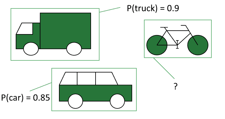
In this sense, labels are a way to compress the complexity of a world into a limited search space, on which we can then work through machine learning.
4. Conclusions
In this tutorial, we’ve seen what are the classes of features that typically appear in datasets for machine learning. We’ve also seen how similar they are to labels. In doing so, we’ve expressed how our judgment is the ultimate thing that distinguishes between the two.
We’ve also seen how labeling data implies a prejudice on the way in which the world operates. In turn, we can treat this prejudice as a Bayesian apriori of the machine learning model. In doing so, we can take benefit, rather than become limited, by our prior knowledge on a given phenomenon.