Understanding Dimensions in CNNs

1. Overview

In this tutorial, we’ll learn how different dimensions are used in convolutional neural networks.

To better grasp these concepts, we’ll illustrate the theory with a few cases from real life. Let’s begin!

2. Convolutions

2.1. Definition

Convolutional Neural Networks (CNNs) are neural networks whose layers are transformed using convolutions.

A convolution requires a kernel, which is a matrix that moves over the input data and performs the dot product with the overlapping input region, obtaining an activation value for every region.

A kernel represents a pattern, and the activation represents how well the overlapping region matches that pattern:

2.2. Dimensions

The objects affected by dimensions in convolutional neural networks are:

• Input layer: the dimensions of the input layer size
• Kernel: the dimensions of the kernel size
• Convolution: in what dimensions the kernel can move
• Output layer: the dimensions of the output layer size

3. 1D Input

3.1. Using 1D Convolutions to Smooth Graphs

For 1D input layers, our only choice is:

• Input layer: 1D
• Kernel: 1D
• Convolution: 1D
• Output layer: 1D

A 1D layer is just a list of values, which we can represent with a graph:

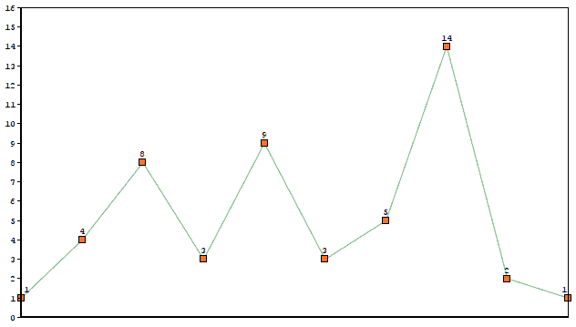
The kernel will slide along the list producing a new 1D layer.

Imagine we used kernel [0.33, 0.67, 0.33] on the previous graph. The output would be:

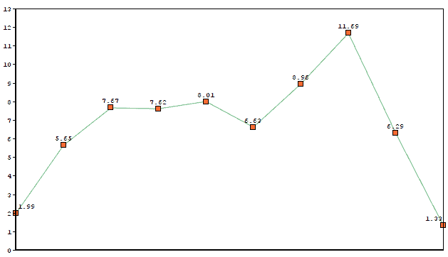
As we see, it still preserves some of the original shape, but now it’s a lot smoother.

4. 2D Input

4.1. Computer Vision with 2D Convolutions

Let’s start with the dimensions:

• Input layer: 2D
• Kernel: 2D
• Convolution: 2D
• Output layer: 2D

This is perhaps the most common example of convolution, where we’re able to capture 2D patterns in images, with increasing complexity as we go deeper in the network:

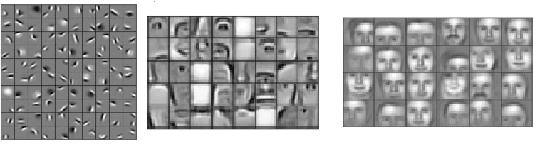
Above we see the kind of patterns a face detection network is able to capture: Earlier layers (left picture) are able to match simple patterns like edges and basic shapes. Middle layers (center picture) find parts of faces like noses, ears, and eyes. Deeper layers (right picture) are able to capture different patterns of faces.

4.2. Encoding n-Grams With 1D Convolutions

In Natural Language Processing, we often represent words with numeric vectors of size , and -gram patterns with kernels. Each activation represents how well those words match the -gram pattern.

Let’s see the dimensions:

• Input layer: 2D
• Kernel: 2D
• Convolution: 1D
• Output layer: 1D

Now imagine that we used a kernel encoding the meaning of “very wealthy”. Most similar words in meaning will have higher activation:

In the example, words like “the richest” produce a high value, as they are similar in meaning to “very wealthy”, whereas words like “is the” return a lower activation.

5. 3D Input

5.1. Finding 3D Patterns with 3D Convolutions

Let’s see what happens when kernel depth < input depth.

Our dimensions are:

• Input layer: 3D
• Kernel: 3D
• Convolution: 3D
• Output layer: 3D

Each 3D kernel is applied over the whole volume, obtaining a new 3D layer:

These convolutions can be used to find tumors in 3D images of the brain, or video events detection, for example.

5.2. Layer Dimensionality Reduction with 2D Convolutions

Now let’s consider the case when kernel depth = input depth.

In that case, our dimensions will be:

• Input layer: 3D
• Kernel: 3D
• Convolution: 2D
• Output layer: 2D

We’ll apply a 3D kernel to a 3D volume in just 2 dimensions because depths match. Et voilá! Now we have a new layer with the same height and width but with one less dimension (from 3D to 2D):

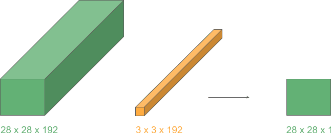
This operation lets us transition between layers of different dimensions and is very often used with height and width 1 for greater efficiency, as we’ll see in the next example.

5.3. Reduce Volume Depth with 1D Kernels

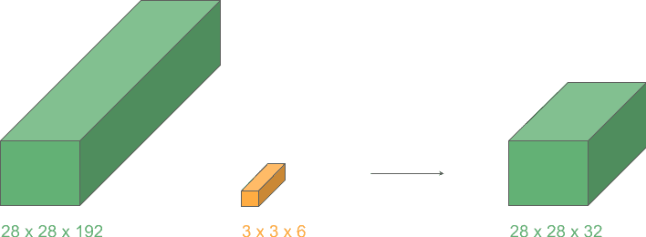
Finally, we’ll take advantage of what we learned in the previous case to create a cool reduction effect.

These are the dimensions:

• Input layer: 3D
• Kernel: 1D
• Convolution: 2D
• Output layer: 3D

From the previous example, we know that applying a 2D convolution to a 3D input where depths match will produce a 2D layer.

Now, if we repeat this operation for kernels, we can stack the output layers and obtain a 3D volume with the reduced depth, .

Let’s see an example of a depth reduction from 192 to 32:

This operation lets us shrink the number of channels in the input, in contrast to typical convolutions where just height and width get reduced. They are widely used in the very popular Google network “Inception”.

6. Conclusion

In this article, we’ve seen the effect of using different dimensions in convolutional objects, and how they are used for different purposes in real life.