Introduction to Convolutional Neural Networks | Baeldung on Computer Science

1. Overview

In this tutorial, we’re going to study the theory behind convolutional neural networks and their architecture.

We’ll start by discussing the task normally performed with convolutional neural networks (CNNs) and the problem of feature extraction. We’ll then discuss why CNNs are required and why traditional feedforward neural networks do not suffice.

We’ll then discuss the operation of convolution in the context of matrix operations. This will give us a good understanding of the mechanisms through which convolutional neural networks operate.

Lastly, we’ll discuss the characteristics of convolutional neural networks other than convolutional layers, with a focus on pooling and dropout.

At the end of this tutorial, we’ll know what a convolutional neural network is and what problems it solves.

2. When Do We Use CNNs

2.1. Why Is Image Recognition So Difficult?

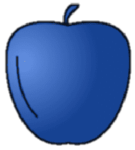
CNNs are used to solve a particular class of problem that consists of the extraction and identification of abstract features in a dataset. Let’s see what this means in practice through a simple example:

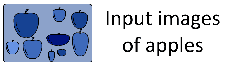
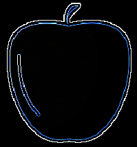
We can see that all images contained in the picture above represent apples of different shapes, sizes, and colors. A human would have no difficulty in identifying them as apples, notwithstanding their slight differences. To a computer, though, the images would appear to be quite different from one another:

These images, however similar they may look to a human, have barely if any points in common to a computer. This is because that which to a human appears as a clearly defined object, to a computer is only a collection of numbers. The human perceptual system in fact uses contextual clues to identify objects, but these, unfortunately, aren’t available to computers.

This means that computers need to rely exclusively on data in order to perform tasks such as the recognition of objects in images. This data can vary however wildly, as we saw in the sample images above. How can we then build a system that works with data that varies so much?

2.2. The Solution Is Abstraction

The task of recognizing apples was made difficult by the fact that too many pixels can assume too many values. And yet, each of them individually carries very little information. This means that an image is highly entropic and that we can’t work with it unless we somehow reduce this entropy significantly.

However, if we had a way to learn abstract features of the input, this would, in turn, make classification sensibly easier. Let’s imagine that we could describe an apple as an object that has a stem, plus a sufficiently flat base, plus, of course, a round shape:

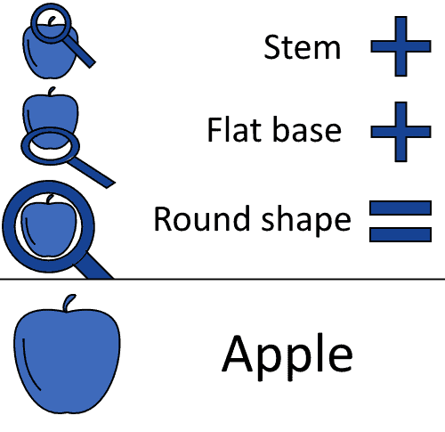
If we could encode these features in a classification algorithm, this would in turn make the classification of unseen images easier. We could, in this case, create a model that encodes the features that we’re looking for, and classify as “apple” an image that possesses them all:

Convolutional neural networks work in this manner; only, they can learn these features automatically. They are, in fact, a way to algorithmically learn abstract representations of a dataset. This, in turn, facilitates the task of classification and helps solve the so-called curse of dimensionality, as we’ll see shortly.

3. Neural Networks and Their Curses

3.1. The Problem That CNNs Address

As per the tradition of our introductory articles on subjects related to machine learning, we’re also going to start studying Convolutional Neural Networks (hereafter, CNNs) with a small analysis of the prior or implicit knowledge which is embedded in this machine learning model. This is best explained by asking ourselves the question:

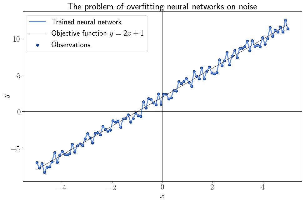
“Why don’t we simply use feedforward neural networks for image classification?”

We know in fact that feedforward neural networks can approximate any continuous function of the form $f: X \in \mathbs{R}^n \to Y \in \mathbs{R}^m$ . There is however no guarantee that neural networks can learn that function. As a general rule, in case we have doubts, it’s safe to assume that a neural network will overfit on the noise of its training data and never learn any given objective function:

3.2. Convolution and Regularization

The attempts at reducing the noise in datasets for the training of neural networks take the name of regularization. Convolution is a particular type of regularization that exploits the linear dependence of features or observations. This, in turn, lets us decrease the noise and restore consistency with the prior assumption on linear independence of the features, as we’ll see shortly.

In broad terms, regularization consists of the mapping of the features of a dataset to new features possessing lower entropy. In formal terms, this means that we transform the features $X \to X\prime$ , such that if $H(X)$ is the entropy of $X$ , then $H(X) \leq H(X\prime)$ . This lets us learn a new objective function $g: f(X) \to g(X\prime)$ that’s less susceptible to overfitting:

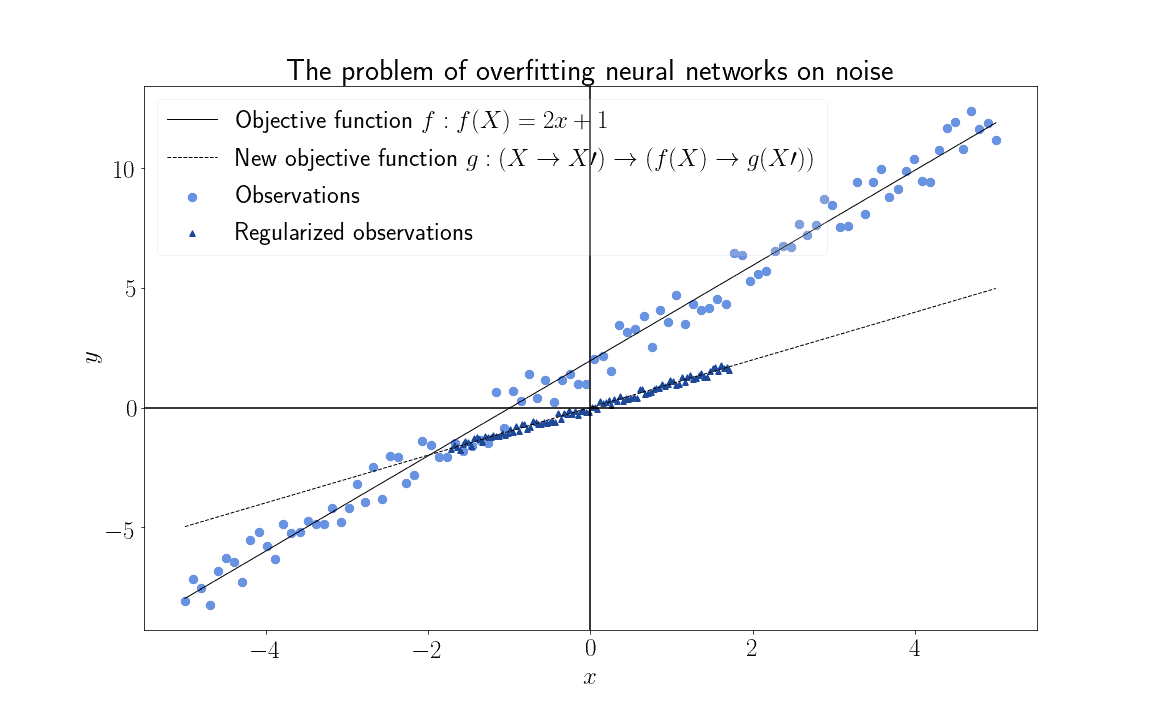
Convolution essentially performs this task, by replacing highly-entropic features in observations with a more complex version of them. This is made possible by the fact that an important precondition for the usage of neural networks, the linear independence of the features, is systematically violated for some classes of data.

3.3. Linear (In)Dependence of Features

Let’s now see in more detail what we mean by features being linearly independent. We can do so with an example by extending to the third dimension the modeling of the distribution of the two variables $X$ and $Y$ , described above.

For that example, we have imagined that a linear relationship existed between the two variables, such that one could be approximated by the other with a function of the form $y = f(x)$ . In particular, we assumed this function to have the form of $Y = 2 X + 1$ , with arbitrarily chosen parameters. We can, therefore, say that, by construction, these two variables are linearly dependent.

Let’s now see what happens if we use two linearly dependent variables as input to some objective function $Z = g(X; Y)$ . The animation below shows the training data sampled from an objective function of the form $Z = g(X; Y) = (\beta_x X+\beta_y Y + \beta_{\epsilon})^2$ :

3.4. Turning Dependent Features Into Independent

For the specific distribution shown in the image, we assigned the values $\beta = \{\beta_x = 1; \beta_y = 1; \beta_{\epsilon}=0\}$ but this is only for explication purposes.

With regards to the structure of the model that we’ll use for regression, we can aprioristically predict some of its characterisitcs. We know that the objective function has quadratic form, because $Z = g(X; Y) = (X+Y)^2 = X^2 + 2XY + Y^2$ . Since $Y$ is linearly dependent $g(X; f(X)) = g(X; 2X + 1)$ .

We can now imagine performing polynomial regression over this function in order to learn its parameters. If we don’t replace $Y$ with its equivalent $f(X)$ , we then have to learn five parameters for our model: $\beta = \{\beta_x; \beta_{x^2}; \beta_y; \beta_{y^2}; \beta_{\epsilon}\}$ . Since the two features $X$ and $Y$ aren’t linearly independent, though, their linear combination is also not linearly independent.

This means that, instead of learning the parameters for the two input variables $X$ and $Y$ , we can instead learn a single set of parameters that corresponds to their linear combination. We can, therefore, learn the more simple model containing the parameters $\beta\prime = \{\beta{\prime}_{(x;y)}; \beta{\prime}_{(x^2;y^2)};\beta{\prime}_{\epsilon}\}$ . This algebraically corresponds to learning the representation of the function on the projected vector space $V_{(X; Y; Z)} \to V_{(X+Y; Z)}$ :

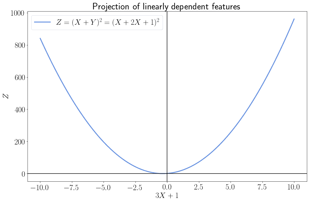
As we can see, we don’t need two input features in this particular example, only one. This is because we had prior knowledge of the linear dependence on the input features. In turn, this prior knowledge lets us reduce the dimensionality of the input to our model, along with its parameters, without any loss in representativity by means of an algebraic transformation.

3.5. The Curse of Dimensionality

This means that, if we have good reasons to believe that the input features to a model aren’t linearly independent, we can decrease the number of parameters that a model requires. This is done by exploiting our prior knowledge on the fact that some classes of data, but not all, possess features that are, at the same time, high dimensional and linearly dependent from one another.

The data that is normally treated with CNNs is typically characterized by a high degree of linear dependency in its features. The most common examples of these are text, audio, image, and video signals:

For text data, the features are normally words, and each of them depends greatly on the ones before and after it
For audio, the frequency varies continuously most of the time
Images are instead a collection of pixels corresponding to colors, where each color is most of the time the same as one of the pixels around it
Videos are a sequence of images, and if they contain real-world information these images only change partially due to object permanence

All these types of data are suitable to be treated with CNNs for the purpose of decreasing their dimensionality. Data with features that we presume to be linearly independent, such as datasets on the characteristics of engines, aren’t instead suitable for CNNs.

3.6. Advantages of CNNs

By using CNNs on highly dimensional data we can help solve the curse of dimensionality in neural networks. This problem refers to the tendency by neural networks to increase the size of their parameters significantly faster than the increase in the size of their input.

We noted in the example above how, for the specific problem of polynomial regression, it was possible to decrease the number of parameters required by 40%. For real-world problems, this decrease is significantly higher, making the usage of techniques for dimensionality reduction, such as convolution, a necessity rather than a choice.

4. Convolution in Neural Networks

4.1. The Mathematical Definition of Convolution

We now understand that, if our data is both linearly dependent and characterized by high dimensionality, we need to use methods for decreasing its entropy. One such method is convolution, which is the operation from which CNNs take their name.

The formula for convolution in neural networks requires the identification of the input data. This is done by first assigning the data (say, an image) on which we perform convolution to a matrix $A_{x,y}$ of dimensionality $(x,y)$ . Then, we define a kernel matrix $k$ whose elements influence the type of result that we obtain from the convolution, as we’ll see in the next section.

The operation of convolution is then defined as the value of an element in the matrix $A$ and all of its local neighbors, multiplied by the corresponding elements in the kernel matrix $k$ :

$k*A = \sum^{x-1}_{i=0} \sum^{y-1}_{j=0} k_{(x-i)(y-j)}A_{(1+i)(1+j)}$

4.2. What Convolution Does to a Matrix

Let’s now see what convolution does to an image, in practice. For this purpose, we’ll use a sample image and see how it changes if we vary the kernel $k$ :

This image is composed of an array of pixels on which we can apply convolution, by defining first a kernel matrix. Various kernels exist that can be used for different purposes. Here we’ll see some, starting with the kernel for blurring:

$k = \frac{1}{9} \begin{bmatrix} \ \ 1 &\ \ 1 &\ \ 1 \\ \ \ 1 &\ \ 1 &\ \ 1 \\ \ \ 1 &\ \ 1 &\ \ 1 \end{bmatrix}$

Another kernel is the one for edge detection:

$k = \begin{bmatrix} \ \ -1 &\ \ -1 &\ \ -1 \\ \ \ -1 &\ \ 8 &\ \ -1 \\ \ \ -1 &\ \ -1 &\ \ -1 \end{bmatrix}$

And another one is the kernel for the sharpening of features:

$k = \begin{bmatrix} \ \ 0 &\ \ -1 &\ \ 0 \\ \ \ -1 &\ \ 5 &\ \ -1 \\ \ \ 0 &\ \ -1 &\ \ 0 \end{bmatrix}$

Different kernels for convolution allow for the extraction of different features from the same data, which in turn helps the training of the CNN. While convolution is the most typical operation of a CNN, from which the architecture itself takes its name, it’s not however the only peculiar characteristic that this network has.

5. Other Characteristics of Convolutional Neural Networks

5.1. General Architecture of CNNs

Despite being called “convolutional” neural networks, CNNs are also characterized by some peculiar features that have nothing to do with convolution. The primary features of CNNs that distinguish them from feedforward neural networks are:

Pooling layers
Dropout layers
And also some special activation functions

A typical architecture for a CNN generally includes a sequence of convolutional, pooling, and dropout layers repeated as many times as necessary. The last layer is then a classification or regression layer, according to the task that we’re performing.

Let’s see a short description of the first two, in order. We can refer to our tutorial on ReLU as an activation function for CNNs for a discussion of the last point.

5.2. Pooling Layers

A peculiar characteristic of CNNs is the pooling layer, which conducts the homonymous mathematical operation of pooling. Pooling consists of the extraction from a given matrix of a new matrix with lower dimensionality, and which contains only one element for each cluster or neighborhood of the original matrix. The most common method for pooling is the so-called Max-Pooling, which works as follows.

We take a matrix $A_{x,y}$ as done before, which represents an image or other input data. We then partition the matrix into neighborhoods of a fixed size. In this case we selected pooling between four elements distributed in a $(2,2)$ pooling window:

$A = \begin{bmatrix} \ \ 1 &\ \ 2 &\ \ 3 \\ \ \ 6 &\ \ 5 &\ \ 4 \\ \ \ 3 &\ \ 1 &\ \ 2 \end{bmatrix} \rightarrow \begin{matrix} \begin{bmatrix} \ \ 1 &\ \ 2 \\ \ \ 6 &\ \ 5 \\ \end{bmatrix} & \begin{bmatrix} \ \ 2 &\ \ 3 \\ \ \ 5 &\ \ 4 \\ \end{bmatrix} \\ \begin{bmatrix} \ \ 6 &\ \ 5 \\ \ \ 3 &\ \ 2 \\ \end{bmatrix}& \begin{bmatrix} \ \ 5 &\ \ 4 \\ \ \ 2 &\ \ 1 \\ \end{bmatrix} \end{matrix}$

We then identify the greatest element among those in a given neighborhood and assign it to the new matrix which we are creating for this purpose:

$\begin{matrix} \begin{bmatrix} \ \ 1 &\ \ 2 \\ \ \ \textbf{6} &\ \ 5 \\ \end{bmatrix} & \begin{bmatrix} \ \ 2 &\ \ 3 \\ \ \ \textbf{5} &\ \ 4 \\ \end{bmatrix} \\ \begin{bmatrix} \ \ \textbf{6} &\ \ 5 \\ \ \ 3 &\ \ 2 \\ \end{bmatrix}& \begin{bmatrix} \ \ \textbf{5} &\ \ 4 \\ \ \ 2 &\ \ 1 \\ \end{bmatrix} \end{matrix} \rightarrow \begin{bmatrix} \ \ 6 &\ \ 5 \\ \ \ 6 &\ \ 5 \\ \end{bmatrix} = {MaxPool}(A)$

The result is a new matrix comprised of only the greatest values among those of the neighbors in the original matrix. This decreases the dimensionality of the input data to a level that makes it more manageable, even though we lose information content as a consequence. The tradeoff is however justified by the linear dependence of the input features, as discussed above.

5.3. Dropout Layers

Convolutional neural networks also implement the so-called Dropout layers, that introduce the capacity to forget into a machine learning model. This is based on the idea that excessive amounts of prior knowledge on a phenomenon may actually hinder, rather than support, the acquisition of future knowledge on that same subject.

Dropout layers work by randomly deactivating some neurons in a given layer, thus forcing the network to adapt to learn with a less-informative signal. While counterintuitive, it has been demonstrated that convolutional neural networks with dropout layers generally learn better when the high-order interactions are spurious. This is because the nullification of part of the signal favors the learning of its abstract features, represented in the higher layers of the network.

For a given dropout parameter $d: 0 \leq d \leq 1$ , we obtain the output of the Dropout function by randomly assigning the value of 0 to each element $a_{i,j}$ of a matrix $A$ with probability $P(0|a_{i,j})=d$ . If $D = {Dropout} (A, d)$ , then formally:

$\forall{i}\forall{j}\forall{a_{i,j} \in A}: [P(D_{i,j} \triangleq 0) = d; P(D_{i,j} \triangleq a_{i,j}) = (1-d)]$

If we take as an example the matrix $A$ from the previous section, and the probability for dropout $d = 0.4$ , we could get this output:

$Dropout (A, d) \to Dropout(\begin{bmatrix} \ \ 1 &\ \ 2 &\ \ 3 \\ \ \ 6 &\ \ 5 &\ \ 4 \\ \ \ 3 &\ \ 1 &\ \ 2 \end{bmatrix}, d=0.4) = \begin{bmatrix} \ \ 0 &\ \ 0 &\ \ 3 \\ \ \ 6 &\ \ 5 &\ \ 0 \\ \ \ 3 &\ \ 0 &\ \ 2 \end{bmatrix}$

The pattern that we would learn over this partially nullified matrix is then less sensitive to overfitting.

6. Conclusions

In this tutorial, we studied the main characteristics of convolutional neural networks.

We started by studying the problem of dimensionality and linear independence of the input features that CNNs address. We then studied convolution as a mathematical operation since this is the operation that most characterizes CNNs. In this context, we also studied what typical kernels we can use for some very common tasks of convolution.

Lastly, we studied the characteristics of CNNs other than their convolutional layers. We learned in particular what pooling and dropout layers are and how they function.

Full Archive

About Baeldung

Core Concepts

Operating Systems

Artificial Intelligence

Graph Theory

Latex