

Learn through the super-clean Baeldung Pro experience:
>> Membership and Baeldung Pro.
No ads, dark-mode and 6 months free of IntelliJ Idea Ultimate to start with.
Learn through the super-clean Baeldung Pro experience:
>> Membership and Baeldung Pro.
No ads, dark-mode and 6 months free of IntelliJ Idea Ultimate to start with.
In this tutorial, we’ll study the similarities and differences between linear and logistic regression.
We’ll start by first studying the idea of regression in general. In this manner, we’ll see the way in which regression relates to the reductionist approach in science.
We’ll then study, in order, linear regression and logistic regression. We’ll also propose the formalization of the two regression methods in terms of feature vectors and target variables.
Lastly, we’ll study the primary differences between the two methods for performing regression over observables. At the end of this tutorial, we’ll then understand the conditions under which we prefer one method over the other.
There’s an idea in the philosophy of science that says that the world follows rules of a precise and mathematical nature. This idea is as old as both philosophy and science and dates back to Pythagoras who attempted to reduce the complexity of the world to relationships between numbers. In modern times, this idea assumed the name of reductionism and indicates the attempts to extract rules and patterns that connect observations with one another.
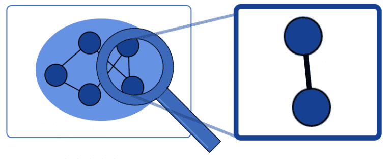
The implicit assumption under reductionism is that it’s possible to study the behavior of subsystems of a system independently from the overall behavior of the whole, broader system:
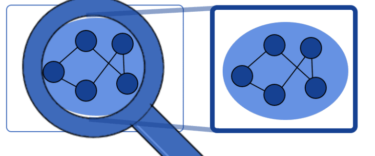
The opposite idea to that of reductionism is called emergence and states, instead, that we can only study a given system holistically. This means that, no matter how accurate we are in summing up and independently analyzing the behavior of the system’s components, we’ll never understand the system as a whole:
Reductionism is a powerful epistemological tool and suitable for research applications in drug discovery, statistical mechanics, and some branches of biology. Reductionism isn’t appropriate for the study of complex systems, such as societies, Bayesian networks for knowledge reasoning, other branches of biology.
We can methodologically treat under regression analysis any problem that we can frame under reductionism, but if we can’t do the latter then we also can’t do the former.
After discussing the epistemological preconditions of regression analysis, we can now see why do we call it in that manner anyway. The word regression, in its general meaning, indicates the descent of a system into a status that is simpler than the one held before. From this, we can get a first intuition that frames regression as the reduction of the complexity of a system into a more simple form.
A second intuition may come by studying the origin, or rather the first usage of the term in statistical analysis. While studying the height of families of particularly tall people, Galton noticed that the nephews of those people systematically tended to be of average height, not taller. This led to the idea that variables, such as height, tended to regress towards the average when given enough time.
As of today, regression analysis is a proper branch of statistical analysis. The discipline concerns itself with the study of models that extract simplified relationships from sets of distributions. Linear and logistic regression, the two subjects of this tutorial, are two such models for regression analysis.
We can conduct a regression analysis over any two or more sets of variables, regardless of the way in which these are distributed. The variables for regression analysis have to comprise of the same number of observations, but can otherwise have any size or content. That is to say, we’re not limited to conduct regression analysis over scalars, but we can use ordinal or categorical variables as well.
The specific type of model that we elect to use is influenced, as we’ll see later, by the type of variables on which we are working. But regardless of this, regression analysis is always possible if we have two or more variables.
Of these variables, one of them is called dependent. We imagine that all other variables take the name of “independent variables”, and that a causal relationship exists between the independent and the dependent variables. Or, at the very least, we suspect this relationship to exist and we want to test our suspicions.
In other words, if  describes a dependent variable and
  a vector containing the features of a dataset, we assume that there exists a relationship
  between these two. Regression analysis then lets us test whether this hypothesis is true.
We can also imagine this relationship to be parametric, in the sense that it also depends on terms other than . In this case, we can denote these terms as  or
or  and call them “parameters” of the regression. In this case, the function
  then assumes the form
  .
.
Lastly, we can also imagine that the measurements from which we derived the values of and are characterized by measurement errors. We discussed the problem of systematic error in measurements in our article on the biases for neural networks; but here we refer to random, not systematic, types of error. We can then call this error  and treat it as causally-independent from the variables that we observe.
We can finally construct a basic model for the relationship between variables that we study under regression analysis. We can thus define:
 , which refers to the -th observation in a dataset, which refers to a dependent variable, which contains independent variables
 , which contains a set of parameters for the model which indicates the random error associated with a given observation
Under these definitions, regression analysis identifies the function such that  .
.
Regression analysis can tell us whether two or more variables are numerically related to one another. However, it doesn’t say anything about the validity of the causal relationship that we presume to exist between them. Simply put, we postulate the assumption of causality before we even undertake regression analysis.
If we find a good regression model, this is sometimes evidence in favor of causality. In that case, we can then say that maybe the variables that we study are causally related to one another.
If we don’t find a well-fitting model, we normally assume that no causal relationship exists between them. However, the scientific literature is full of examples of variables that were believed to be causally related whereas they in fact weren’t, and vice versa.
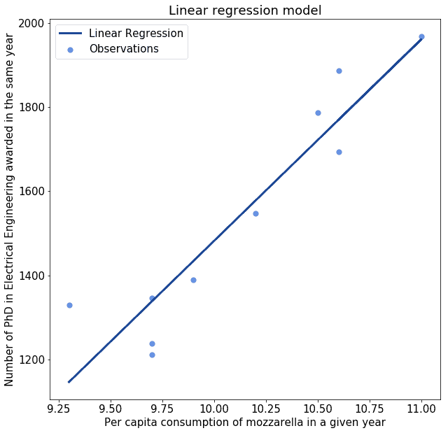
It’s therefore extremely important to keep in mind the following. Having a good regression model over some variables doesn’t necessarily guarantee that these two variables are related causally. If we don’t keep this in mind, we then risk assigning causality to phenomena that are clearly unrelated:
Let’s suppose that the two variables  that we’re studying have equal dimensionality, such that
  . Let’s now imagine that a linear relationship exists between
  and , which implies the existence of two parameters
  , such that
  . The relationship is perfectly linear if, for any element
  of the variable , then
  .
.
We can formalize the previous statement by saying that a model is linear if:

Notice how if  , this implies that
  independently of any values of . The question of whether
  is true or false, then is independent of . This means that for we’re no longer talking about two variables, but only one.
We can, therefore, say that the model is undefined for that parameter  , but for all other values of
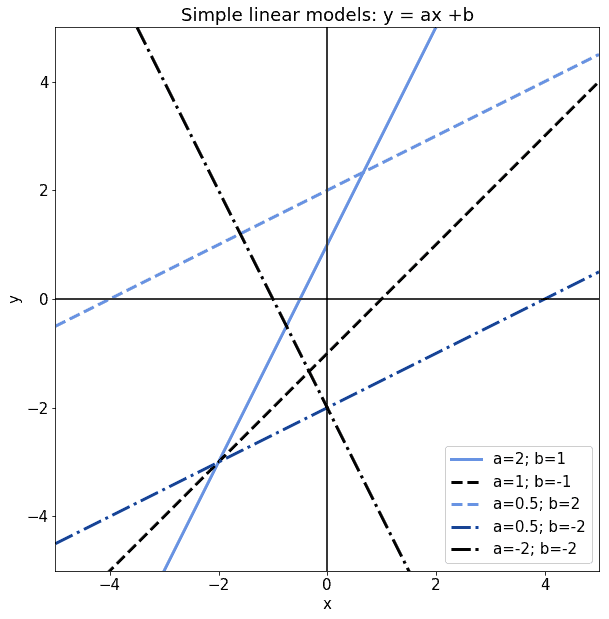
  the model is otherwise defined. The following are all valid examples of linear models with different values for their and
  parameters:
Let’s now imagine that the model doesn’t fit perfectly. This means that, if we calculate for a given its associated linearly-paired value  , then there’s at least one such that
  .
.
In this case, we can compute a so-called error between  , the prediction of our linear model, and
  , the observed value of the variable. We can call this error
  .
.
The problem of identifying a simple linear regression model consists then in identifying the two parameters  of a linear function, such that
  . The additional constraint is that we want this error term to be as small as possible, according to some kind of error metric.
The typical error metric used in linear regression is the sum of the squared errors, which is computed as:

The problem of identifying the linear regression model for two variables can thus be reformulated as the finding of the parameters which minimize the sum of squared errors. In other words, the problem becomes the identification of the solution to:

The solution to this problem can be found easily. We can compute first the parameter , as:

where  and
and  are the average values for the variables and . After we find , we can then identify simply as:
  . The two parameters that we have thus computed, correspond to the parameters of the model
  that minimize the sum of squared errors.
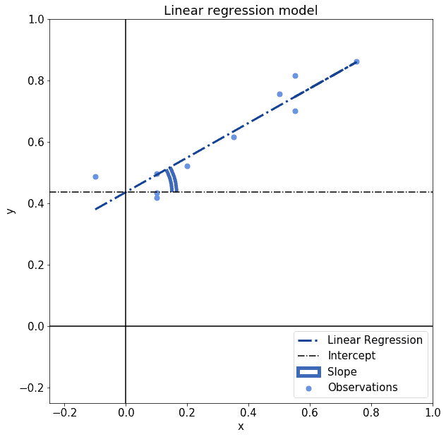
There’s also an intuitive understanding that we can assign to the two parameters , by taking into account that they refer to a linear model. In linear regression, as well as in their related linear model, and refer respectively to the slope of a line and to its intercept:
Lastly, in the specific context of regression analysis, we can also imagine the parameter as being related to the correlation coefficient  of the distributions and , according to the formula
  . In this formula,
  and
and  refer respectively to the uncorrected standard deviations of and . Correlation is, in fact, another way to refer to the slope of the linear regression model over two standardized distributions.
We can now state the formula for a logistic function, as we did before for the linear functions, and then see how to extend it in order to conduct regression analysis. As was the case for linear regression, logistic regression constitutes, in fact, the attempt to find the parameters for a model that would map the relationship between two variables to a logistic function.
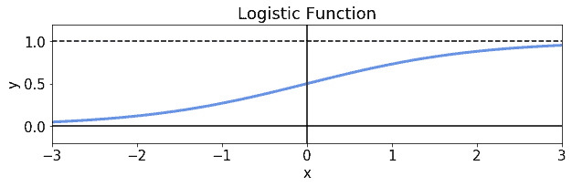
A logistic function is a function of the form  , where indicates Euler’s number and is, as was before the the linear model, an independent variable. This function allows the mapping of any continuously distributed variable
  to the open interval
  . The graph associated with the logistic function is this:
The logistic function that we’re showing is a type of sigmoidal function. The latter is particularly important in the context of non-linear activation functions for neural networks. It’s also, however, the basis for the definition of the Logit model, which is the one that we attempt to learn while conducting logistic regression, as we’ll see shortly.
Since the codomain of the logistic function is the interval , this makes the logistic function particularly suitable for representing probabilities. While other uses of the logistic function also exist, the function is however typically employed to map real values to Bernoulli-distributed variables.
If a dependent variable is Bernoulli-distributed, this means that it can assume one of two values, typically 0 and 1. The input to the logistic function, instead, can be any real number. This makes the logistic function particularly adapted for applications where we need to compress a variable with domain  to a finite interval.
Because we can presume the dependent variable in a logistic model to be Bernoulli-distributed, this means that the model is particularly suitable for classification tasks. In that context, the value of 1 corresponds to a positive class affiliation. Symmetrically, the value of zero corresponds to the incorrect classification. This makes, in turn, the logistic model suitable for conducting machine-learning tasks that involve unordered categorical variables.
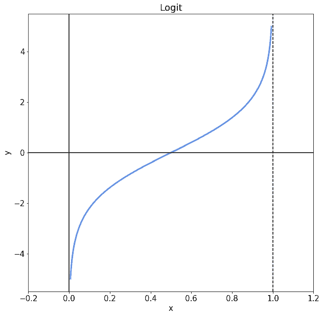
After defining the logistic function, we can now define the Logit model that we commonly use for classification tasks in machine learning, as the inverse of the logistic function. In other words, this means that:

The Logit model is the link model between a Bernoulli-distributed variable and a generalized linear model. A generalized linear model is a model of the form  . This corresponds laregely to the linear model we studied above.
In that model, as in here, is a vector of parameters and contains the independent variables. A link function such as Logit then relates a distribution, in this case, the Binomial distribution, to the generalized linear model.
In using the Logit model, we receive a real value that returns a positive output over a certain threshold for the model’s input. This, in turn, triggers the classification:
The question now becomes, how do we learn the parameters of the generalized linear model? In the case of logistic regression, this is normally done by means of maximum likelihood estimation, which we conduct through gradient descent.
We define the likelihood function  by extending the formula above for the logistic function. If is the vector that contains that function’s parameters, then:

We can then continue the regression by maximizing the logarithm of this function. The reason has to do with the monotonicity of the logarithm function. This monotonicity, in fact, implies that its maximum is located at the same value of that logarithm’s argument:

The function  also takes the name of log-likelihood. We can now identify this maximum to an arbitrary degree of precision with a step-by-step process of backtracking. This is because, in correspondence to the maximum of the log-likelihood, the gradient is zero. This means that the values of the parameters that satisfy this condition can be found by repeatedly backtracking until we’re satisfied with the approximation.
We can now sum up the considerations made in this article. This lets us identify the primary differences between the two types of regression. Specifically, the main differences between the two models are:
 , while logistic regression implies
 , whereas logistic regression has a codomain of
 The similarities, instead, are those that the two regression models have in common with general models for regression analysis. We discussed these in detail earlier, and we can refer to them in light of our new knowledge.
In this article, we studied the main similarities and differences between linear and logistic regression.
We started by analyzing the characteristics of all regression models and to regression analysis in general.
Then, we defined linear models and linear regression, and the way to learn the parameters associated with them. We do this by means of minimization of the sum of squared errors.
In an analogous manner, we also defined the logistic function, the Logit model, and logistic regression. We also learned about maximum likelihood and the way to estimate the parameters for logistic regression through gradient descent.
Finally, we identified in a short form the main differences between the two models. These differences related to both their peculiar characteristics and their different usages.