

Learn through the super-clean Baeldung Pro experience:
>> Membership and Baeldung Pro.
No ads, dark-mode and 6 months free of IntelliJ Idea Ultimate to start with.
Learn through the super-clean Baeldung Pro experience:
>> Membership and Baeldung Pro.
No ads, dark-mode and 6 months free of IntelliJ Idea Ultimate to start with.
In this tutorial, we will discuss the training, validation, and testing aspects of neural networks. These concepts are essential in machine learning and adequately represent the different phases of a model’s maturity. It’s also important to note that these ideas are adjacent to many others, such as cross-validation, batch optimization, and regularization.
The field of machine learning has expanded tremendously thanks to neural networks. These neural nets are employed for a wide variety of reasons because they are very flexible models that can fit almost any kind of data, provided that we have sufficient computing resources to train them in a timely manner. To efficiently exploit these learning structures, we need to make sure that the model generalizes the information that is being processed.
The problem here is that if we feed all the data we have for the model to train, there is no way that we can test if the model has correctly extracted a function from the information. This metric is called accuracy, and it’s essential for assessing the performance of our model.
Alright, we can begin by making a training set and a testing set. We can now train our model and verify its accuracy using the testing set. The model has never seen the test data during training. Therefore, the accuracy result we will obtain will be valid. We can use different techniques to train a neural network model, but the easiest to understand and implement is backpropagation. Now, let’s say that we get a less-than-favorable performance from our training-testing approach. We can maybe change some hyperparameters from our model and try again.
However, if we do so, we will be using the results from the test set to tune the training of the model. There is something wrong with this approach in theory because we are adding a feedback loop from our test set. This will falsify the accuracy results that we will generate because we are changing parameters based on the results we achieve. In other words, we are using the data from the test set to optimize our model.
To avoid this, we perform a sort of “blind test” only at the end. In contrast, to iterate and make changes throughout the development of the model, we use a validation set. Now we can use this validation set to fine-tune various hyperparameters to help the models fit the data. Additionally, this set will act as a sort of index for the actual testing accuracy of the model. This is why having a validation data set is important.
We can now train a model, validate it, and change different hyperparameters to optimize performance and then test the model once to report its results.
Let’s see if we can apply this to an example.
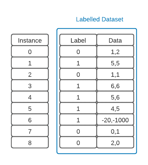
To implement these notions in a classic supervised learning fashion, we must first obtain a labeled data set to work with. An example of one with two classes that use coordinates as a single feature will be represented below:
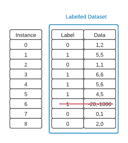
The first thing to note is that there is an outlier in our data. It’s good practice to find these using common statistical methods, examine them, and then remove those that don’t add information to the model. This is part of an important step called data pre-processing:
Now that we have our data ready, we can split it into training, validation, and testing sets. In the figure below, we add a column to our data set, but we could also make three separate sets:
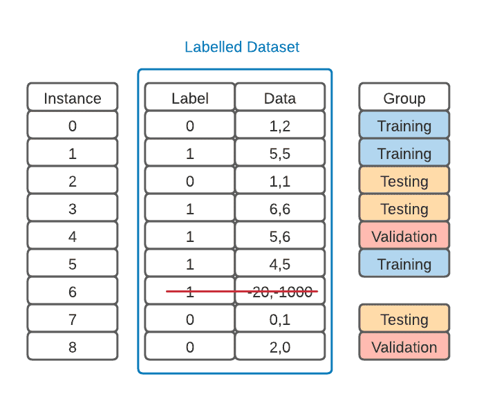
We must ensure that these groups are balanced so that our model is less biased. This means that they must have more or less the same amount of examples from each label. Failure in balancing could lead to the model not having enough examples of a class to learn accurately. This could also put the test results in jeopardy.
In this binary classification example, our training set has two “1” labels and only one “0” label. However, our validation set has one of each, and our testing set has two “0” labels and only one “1” label. Because our data is minimal, this is satisfactory.
However, we could change the groups that we defined and pick the best configuration to see how the model performs in testing. This would be called cross-validation. K-fold cross-validation is widely used in ML. However, it’s not covered in this tutorial.
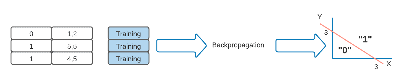
Moving on, we can now train our model. In the case of our feed-forward neural net, we could use a backpropagation algorithm to do so. This algorithm will compute an error for each training example and use it to finely adjust the weights of the connections in our neural net. We run this algorithm for as many iterations as we can until it’s just about to overfit our data, and we get the model below:
In order to verify the correct training of the model, we feed our trained model the validation dataset and ask it to classify the different examples. This will give us validation accuracy.
If we were to have an error in the validation phase, we could change around any hyper-parameters to make the model perform better and try again. Maybe we can add a hidden layer, change our batch size, or even adjust our learning rate depending on the optimization methods.
We can also use the validation dataset for early stopping to prevent the model from overfitting data. This would be a form of regularization. Now that we have a model that we fancy, we simply use the test dataset to report our results, as the validation dataset has already been used to tune the hyper-parameters of our network.
Let’s explore how to implement training, testing, and validation in Python. For that, we’ll use the scikit learn machine learning framework. It’s a free and open-source simple and efficient tool that we can use even for commercial applications. For this practice, we’ll also use its Iris flower dataset. This dataset is quite well-known, it’s a multivariable dataset that uses multiple morphologic measurements to classify flowers fo three related Iris flower species.
There are some online development environments we can use to develop Python code, such as Google Colab. If that is the case, we can go to the next step. However, if we want to work locally, we must set up our development.
There is a good chance that our OS already has Python3 installed by default, however, if not, we must install the Python language. Now, creating a specific Python environment for each project is advisable. This way, project dependencies will not interfere with each other:
$ mkdir my_first_ml_project
$ cd my_first_ml_project
$ python3 -mvenv env
The above commands will create a new directory and an env folder under it that will hold any dependency we need. To activate under Linux or Mac OS X the new environment we must use:
$ . ./env/bin/activateOn Microsoft Windows, the command is:
C:\Users\user\my_first_ml_project> .\env\scripts\activateNow, we can install the dependencies.
First, let’s start with the Jupyter Notebook, an excellent Python web-based IDE that is one of the main tools of any data scientist:
pip install notebookAlso, that is a good time to install the other dependencies we will need:
pip install pandas pyarrow seaborn matplotlib scikit-learnTo run it, we must call it executable: jupyter-notebook. At the end, it’ll show its web access URL.
(env) baeldung@host:~/ML$ jupyter-notebook
 ...
    To access the server, open this file in a browser:
        file://Users/guilherme/AppData/Roaming/jupyter/runtime/jpserver-2888-open.html
    Or copy and paste one of these URLs:
        http://localhost:8888/tree?token=d0bce16a9d501e82043e18acd6400a045c461a0f984d9eca
        http://127.0.0.1:8888/tree?token=d0bce16a9d501e82043e18acd6400a045c461a0f984d9eca
[I 2024-02-16 20:41:57.128 ServerApp] Skipped non-installed server(s): bash-language-server, dockerfile-language-server-nodejs, javascript-typescript-langserver, jedi-language-server, julia-language-server, pyright, python-language-server, python-lsp-server, r-languageserver, sql-language-server, texlab, typescript-language-server, unified-language-server, vscode-css-languageserver-bin, vscode-html-languageserver-bin, vscode-json-languageserver-bin, yaml-language-server
The default browser should open automatically, if it doesn’t, we can click on any HTTP URLs to open the Jupyter Notebook on a browser.
We’ll start by taking a glimpse at the Iris dataset. We’ll load it from the Scikit Learn provided datasets. First, we must install the requirements, activate the virtual environment as shown above, the run in the command line:
pip install pandas pyarrow seaborn matplotlib scikit-learnAlternatively, you can do that on the Jupyter Notebook by using the following command on a new Notebook file:
%pip install pandas pyarrow seaborn matplotlib scikit-learn
Now, let’s start our python sample:
# Load libraries
import pandas as pd
import seaborn as sns
from matplotlib import pyplot as plt
Now, let’s import the dataset and prepare it for use:
from sklearn.datasets import load_iris
iris_data = load_iris()
iris = pd.DataFrame(iris_data.data, columns=iris_data.feature_names)

# Add labels
iris['Species'] = list(map( lambda i: iris_data.target_names[i], iris_data.target))
Let’s take a glimpse at the dataset:
sns.pairplot(iris, hue='Species')This will show the following picture:
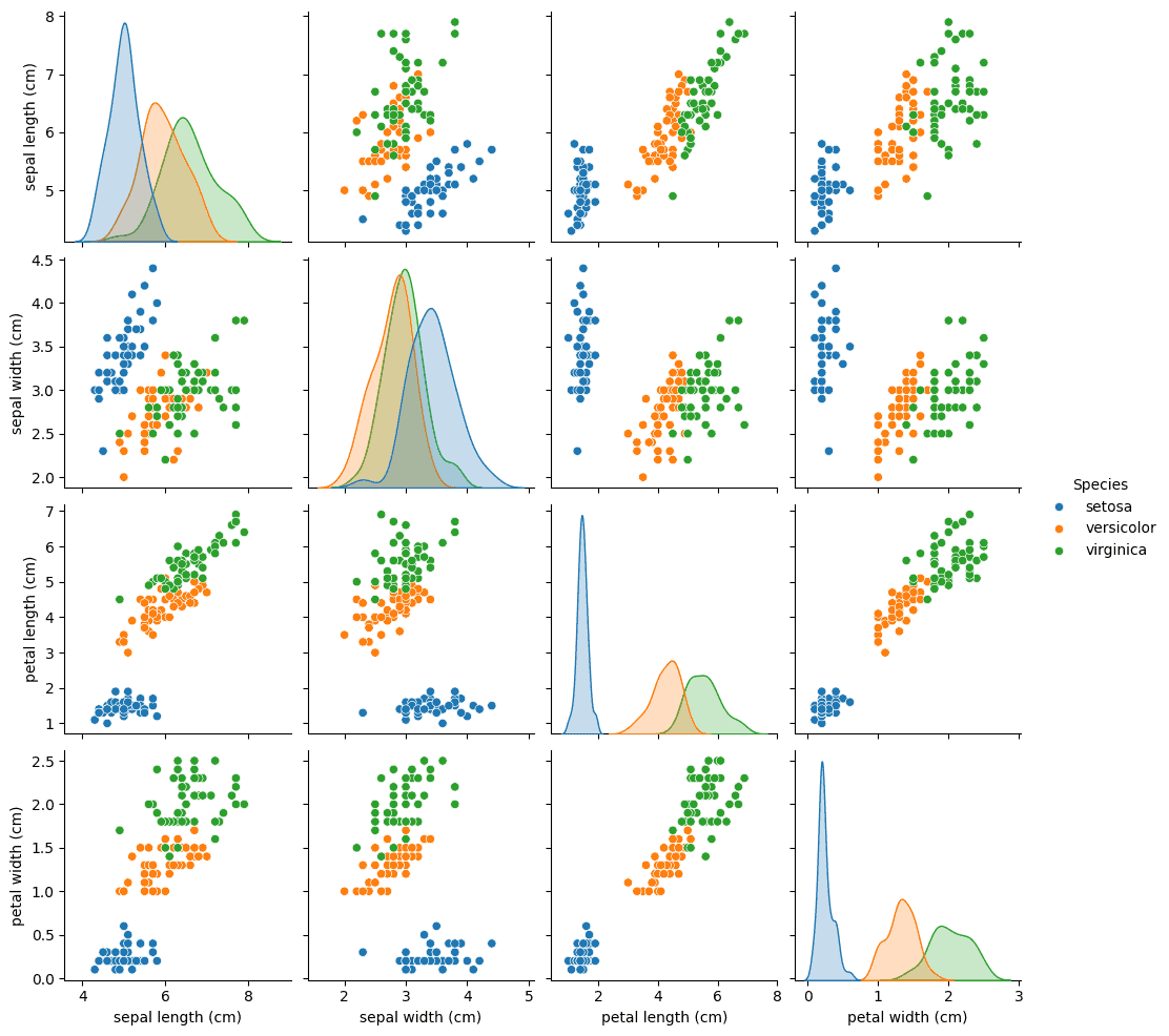
This graph shows how the various flower species can be clustered by each dimension of the dataset. Now, we can train a neural network to, given any set of sepal and petal dimensions, guess the correct species it belongs to.
To split the dataset we’ll use the train_test_split function from Sklearn twice. This function will randomly split a dataset in two using a given ratio. In our tutorial, we’ll use 40% of the data to validate and test.
Import the train_test_split method
from sklearn.model_selection import train_test_splitFirst let’s split the training dataset using 60% of the whole dataset:
validation_test_sizes = 0.4 train, validation_test = train_test_split(iris, test_size = 0.4)
print ("Train:\t\t", train.shape[0], "objects")
Now, let’s split the remaining data samples into the validation and testing datasets:
validation, test = train_test_split(validation_test, test_size = .5)
print ("Validation:\t", validation.shape[0], "objects")
print ("Testing:\t", test.shape[0], "objects")
Finally, let’s prepare the three datasets to use with Sklearn functions:
train_X = train[['sepal length (cm)', 'sepal width (cm)', 'petal length (cm)', 'petal width (cm)']]
train_y = train.Species

validation_X = validation[['sepal length (cm)', 'sepal width (cm)', 'petal length (cm)', 'petal width (cm)']]
validation_y = validation.Species

test_X = test[['sepal length (cm)', 'sepal width (cm)', 'petal length (cm)', 'petal width (cm)']]
test_y = test.SpeciesNow, we can train and validate the neural network model using different hyperparameters. In the following sample, we’ll try different hidden layer sizes:
We will use a Mulit-layered Perceptron Classifier neural network. So, let’s import it:
from sklearn.neural_network import MLPClassifierTo access the quality of the model we will use an accuraccy metric, let’s import it:
from sklearn.metrics import accuracy_score
Train and validate using different hyperparameters, we’ll try different neural networks ranging from 1 to 10 neurons on the hidden layer:
# The hyperparameter we'll change is the number of neurons in the hidden layer, ranging from 1 to 10
best_accuracy = 0
best_model = None
for i, layer_size in enumerate(range(1,11,1)):
    print ('{}: Testing neural network MLP classifier with {} neurons on the hidden layer'.format(i + 1, layer_size))
    model = MLPClassifier(hidden_layer_sizes=layer_size, max_iter=20000)

    # Train
    model.fit(X=train_X, y=train_y)

    # Validate
    p = model.predict(X=validation_X)

    current_accuracy = accuracy_score(p, validation_y)
    print ('\taccuracy using the validation dataset:\t{:.3f}'.format(current_accuracy))

    if best_accuracy < current_accuracy:
        best_model=model
        best_accuracy = current_accuracy

    del (model)
print ('Best model had {} neurons in the hidden layer'.format(best_model.get_params()['hidden_layer_sizes']))
This will print something like this:
1: Testing neural network MLP classifier with 1 neurons on the hidden layer
	accuracy using the validation dataset:	0.900
2: Testing neural network MLP classifier with 2 neurons on the hidden layer
	accuracy using the validation dataset:	0.667
3: Testing neural network MLP classifier with 3 neurons on the hidden layer
	accuracy using the validation dataset:	0.967
4: Testing neural network MLP classifier with 4 neurons on the hidden layer
	accuracy using the validation dataset:	0.800
5: Testing neural network MLP classifier with 5 neurons on the hidden layer
	accuracy using the validation dataset:	1.000
6: Testing neural network MLP classifier with 6 neurons on the hidden layer
	accuracy using the validation dataset:	1.000
7: Testing neural network MLP classifier with 7 neurons on the hidden layer
	accuracy using the validation dataset:	0.967
8: Testing neural network MLP classifier with 8 neurons on the hidden layer
	accuracy using the validation dataset:	1.000
9: Testing neural network MLP classifier with 9 neurons on the hidden layer
	accuracy using the validation dataset:	1.000
10: Testing neural network MLP classifier with 10 neurons on the hidden layer
	accuracy using the validation dataset:	1.000
Best model had 5 neurons in the hidden layer
In this case, the best scenario was with 5 neurons in the hidden layer. We should note that, as the dataset splitting and the training starting weight values are, by default, chosen randomly, other executions may end with different results. This behavior, however, is desirable. Removing the randomness will increase the risk of biased training.
Also, it should be noted that the accuracy was extremely high, 100%. We most likely won’t want that, as it may give a model that is extremely good at classifying known samples but performs poorly with new data, An issue that we call overtraining, and should be avoided.
Once we choose the model with the best accuracy, we can test it:
p = best_model.predict(X=test_X)
best_model_testing_accuracy = accuracy_score(p, test_y)
print ('\taccuracy using the testing dataset:\t{:.3f}'.format(best_model_testing_accuracy))
This will give the following result:
accuracy using the testing dataset: 0.967Now, we can even show the classification report:
from sklearn.metrics import accuracy_score, classification_report

print (classification_report(test_y,p))
Which gives:
              precision    recall  f1-score   support

      setosa       1.00      1.00      1.00        10
  versicolor       1.00      0.92      0.96        12
   virginica       0.89      1.00      0.94         8

    accuracy                           0.97        30
   macro avg       0.96      0.97      0.97        30
weighted avg       0.97      0.97      0.97        30
Or the confusion matrix:
from sklearn.metrics import confusion_matrix, ConfusionMatrixDisplay

cm = confusion_matrix(test_y, p, labels=iris_data.target_names)
cmd= ConfusionMatrixDisplay(cm, display_labels=iris_data.target_names)
cmd.plot()
cmd.ax_.set_title('{}. Accuracy: {:.4f}'.format(best_model, best_model_accuracy))
That shows:
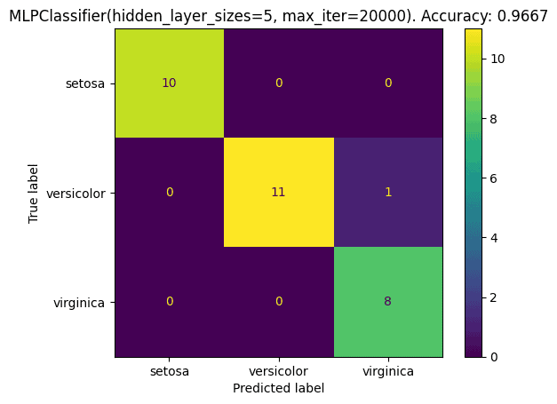
In this case, the validation led to a 96.67% accuracy, with only one misclassification, one versicolor flower was wrongly classified as a virginica.
In this article, we discussed the different notions of training, testing, and validating in machine learning.
We also showed how to implement it in Python using the Scikit Learn toolkit.