Why Does the Cost Function of Logistic Regression Have a Logarithmic Expression?

1. Overview

In this tutorial, we’re going to study the reasons why we use a logarithmic expression for the error function of a logistic regression model.

To do so, we’re first going to discuss the problem of algorithmic learning in general. This will let us know what are the conditions required to guarantee that any given function can be learned through gradient descent.

Subsequently, we’ll define the mathematical formulation of a model for logistic regression. In connection to this, we’ll also define the likelihood function of this model and study its properties. This will let us understand why it’s not guaranteed that, in general, we can always learn that model’s parameters.

Lastly, we’ll study the logarithmic variation of the likelihood function. In doing so, we’ll learn what is the difference between likelihood and log-likelihood in terms of the learnability of their parameters.

At the end of this tutorial, we’ll have a deep theoretical understanding as to the reason why we use a logarithmic function to learn the parameters of a logistic regression model, in relation to the general problem of the learnability of a function.

2. Learning Parameters Through Gradient Descent

2.1. The Problem of Learning Parameters

Before we get into the specificity of logistic regression and its associated error function, it’s important to spend a few words on the subject of algorithmic learning of parameters in models in general. There’s, in fact, a simple explanation as to why we choose a logarithmic function as an error function for logistic models instead of simply mean squared error.

This explanation, however, requires us to understand what characteristics we expect an error function to possess in machine learning models.

There are different ways to learn the parameters in a model. The most famous of these is gradient descent, which is a generalized method for learning the parameters in any continuous and differentiable function. The most common application of gradient descent is in the learning of weights in a neural network. This is because weights can be considered as parameters sui generis of that network.

Gradient descent is also how we learn the parameters for the logistic regression model. It’s in this context that we can study this algorithm then. By learning about the conditions for the application of gradient descent, we’ll also therefore learn the characteristics expected to a function on which we apply this algorithm.

2.2. Gradient Descent and Its Requirements

Gradient descent is an algorithmic way to find a minimum point in a differentiable function that doesn’t require knowledge of the shape of that function but only of its partial derivatives. This algorithm can be applied to any function $f(x)$ and, provided that we satisfy its requirements, guarantees convergence.

This means that if a minimum exists for a function that satisfies some conditions, we can then approximate it to an arbitrary degree of precision. These conditions are:

$f$ is continuous and differentiable in $x$
$f$ is also convex
and lastly, its gradient is Lipschitz-continuous

If a function meets these conditions, we can then find a value $x*$ such that $f(x*) - f(x_0) < \epsilon$ . In here, $x_0$ is the value of $f$ for which $f'(x_0) = 0 \wedge f''(x_0) \geq 0$ . The value $\epsilon$ , indicating the level of approximation, is instead any arbitrarily chosen value.

In other words, this means that if an objective function and its gradient satisfy the conditions listed, we can then always find through gradient descent a point of the function that is as close as we desire to its minimum. We can thus reformulate the problem of choosing a cost function for the logistic regression into the problem of choosing a cost function on which we can apply gradient descent.

3. Logistic Regression

3.1. A Review on the Logistic Function

In our previous article on the difference between linear and logistic regression, we discussed how a logistic model maps a generalized linear function of the form $f(x) = ax + b$ to the open interval $(0,1)$ . This model is, therefore, a continuous mapping of the form $f: \mathbs{R} \to (0,1)$ . The most typical of these maps is the logistic function, which can in turn be written as:

$y = f(x) = \frac {e^{(ax+b)}}{e^{(ax+b)} + 1} = \frac{1}{1+e^{-(ax+b)}}$

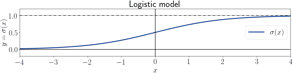
where the generalized linear model has become an exponent for Euler’s number $e$ . This function, if $a=1$ and $b=0$ , acquires the notorious $S$ shape which made it famous:

3.2. Logistic Regression and Generalized Linear Models

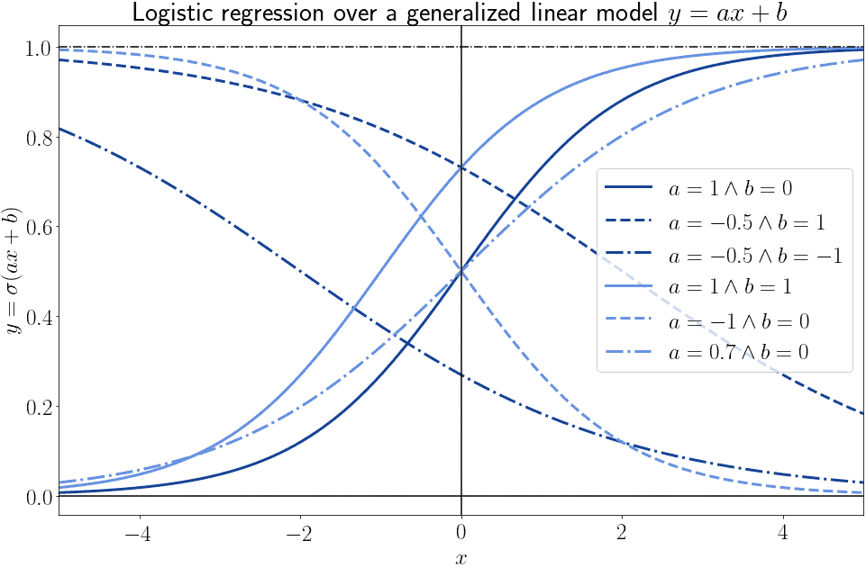
The generalized linear model can however have parameters $a$ and $b$ that differ from the two indicated above. In that case, even though the general $S$ shape is still present, the values assumed by the function can vary wildly. Here we can see some examples of different logistic models with a one-dimensional independent variable:

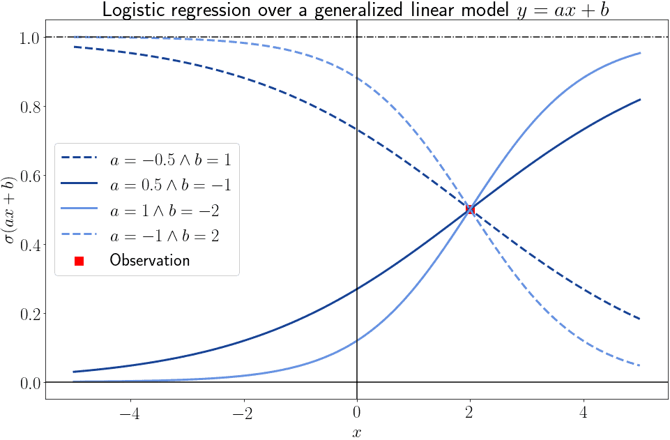
In general, we can affirm that for any point $(x, y): x \in \mathbs{R} \wedge y \in (0,1)$ there are infinite logistic models of the form $y = \sigma(ax+b)$ that pass through that point. Each of them corresponds to a given combination of values for the pair of parameters $(a,b)$ .

3.3. Logistic Regression Against Training Data

This means that, if we only take one observation from those present in a dataset, we can’t really infer much about the parameters of the best-fitting logistic model:

As the number of observations starts to increase, however, we can progressively narrow down the parameters of the model that best fits them. This lets us go down from the many possible models to one best-fitter:

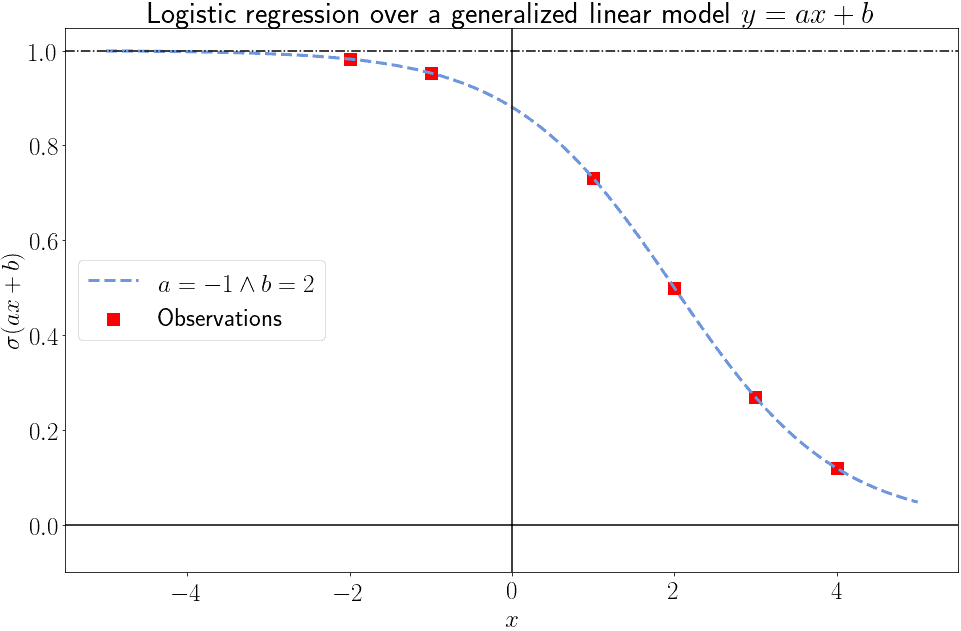
This is, in essence, the idea behind logistic regression. In real-world datasets, however, no single model will perfectly fit any given set of independent and dependent variables. This is due to two main reasons:

the values of variables in real-world datasets are influenced by random errors
the output of the logistic model is a continuous variable included in the domain $(0,1)$ , while the dependent variable that we use for training is a Bernoulli-distributed $y: y = 0 \vee y = 1$

As a consequence of this, we expect even the best-fitting model to have non-zero prediction errors. The problem of finding the parameters for the best-fitting logistic model can then be shifted towards the problem of finding the parameters of the model that minimizes some kind of error metrics. We’ll see shortly what do we mean by that, with regards to various possible error functions.

3.4. The Mathematical Definition of Logistic Regression

We can now sum up the main characteristics of the logistic regression in a more formalized manner. From this, we’ll first build the formal definition of a cost function for a logistic model, and then see how to minimize it.

A logistic model is a mapping of the form $f: (-\infty, \infty) \to (0, 1)$ that we use to model the relationship between a Bernoulli-distributed dependent variable $y: y = 0 \vee y =1$ and a vector $X$ comprised of $n$ independent variables $\{x_1, x_2, ... , x_n\}$ , such that $x \in X \to x_i \in \mathbb{R}$ .

We also presume the function $f$ to refer, in turn, to a generalized linear model $g(X,A)=$ . In here, $X$ is the same vector as before and $A$ indicates the parameters of a linear model over $X$ , such that $A = \{a_0, a_1, ..., a_n\} \to y = a_0 + a_1 x_1 + a_2 x_2 + ... + a_n x_n$ . In this case, we can rewrite $y = f(X)$ as $y = f(g(X,A))$ .

Notice how $|A| = |X|+1$ ; i.e., there’s one more parameter in $A$ than there are variables in $X$ . This is because we can treat the intercept or constant term of a linear model as the coefficient of a variable with exponent zero, since $a_0 = a_0 x^{0} | \forall x, a \in \mathbb{R} \wedge x \neq 0$ . Or, equivalently, we can impose $x = 1$ and obtain the same result.

3.5. Logistic Regression in Parametric Form

We can now write $g(X,A)$ in algebraic form as $g(X,A) = A^{T} X$ , and express $f$ as a logistic function over $g(X,A)$ , as:

$y = f(g(X,A)) = \frac{1}{1+e^{-g(X,A)}}$

By replacing $g(X,A)$ with its algebraic equivalent we can then obtain:

$y = f(g(X,A)) = \frac{1}{1+e^{-A^{T}X}}$

which is the logistic regression in its parametric form. Since $y$ is Bernoulli-distributed, the common interpretation is to consider $f$ as the probability function of $y=1$ given $X$ and $A$ :

$P(y=1|X,A) = f(X,A)$

Since $y$ can only assume the two values of 0 or 1, we can also calculate $P(y=0|X,A)$ as $P(y=0|X,A) =1- f(X,A)$ . For a given observation $k$ , we can then rewrite the probability as:

$P(y_k=0|X_k,A) \times P(y_k=1|X_k,A) = f(X_k,A)(1- f(X_k,A))$

Lastly, we can calculate the likelihood function $L(A | Y, X)$ as $P(Y | X,A)$ , by multiplying over all the observations of the distributions $Y$ and $X$ :

$L(A|y,x) = P(Y|X,A) = \prod_{i}^{n}{P(y_i | x_i, A)}$

If we take into account that $y$ can assume only the values of 0 and 1, we can then rewrite the formula as:

$L(A|y,x) = \prod_{i}^{n}{f_A(x_i)^{y_i}(1-f_A(x_i))^{(1-y_i)}}$

4. Cost Function of the Logistic Regression

4.1. Why Not Using Mean Squared Error?

The problem is now to estimate the parameters $A$ that would minimize the error between the model’s predictions and the target values. In other words, if $h_A(x_i)$ is the prediction of the model for $x_i$ given the parameters $A$ , we want $min(Err(h_A(x),y))$ where $Err$ is the error metric we use.

Let’s now imagine that we apply to this logistic model the same error function that’s typical for linear regression models. This function normally consists of the mean squared error ( $MSE$ ) between the model’s predictions and the values of the target variable. We can write $MSE(x,y|A)$ as:

$MSE(x,y|A) =\frac{1}{n} \sum_{i=1}^{n} h_A(x_i) - y_i)^2$

4.2. The Problem of Convexity

For the case of the linear model, $MSE$ was guaranteed to be convex because it was a linear combination of a prediction function that was also composed. For the case of logistic regression, $MSE$ isn’t guaranteed to be convex because it’s a linear combination between scalars and a function, the logistic function, that’s also not convex.

As an example, this is the general shape of the decision function $h_A(x)$ , for the specific case of $a=1 \wedge b =0$ :

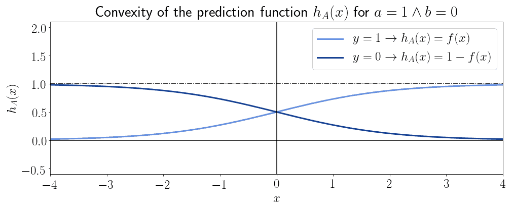
And this is the convexity associated with $h_A(x)$ :

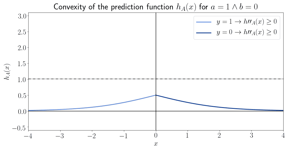
We can see that the decision function isn’t generally convex, but only in a specific subset of its domain.

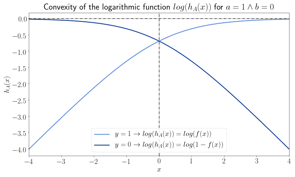
4.3. The Logarithm of the Prediction Function

This means that we can’t use the mean squared error as an error metric for the logistic model. Let’s consider instead the logarithm of the prediction function, $ln(h_A(x_i))$ when $y_i = 1$ , and $ln(1-h_A(x_i))$ when $y_i=0$ . These functions are, interestingly for us, guaranteed to never be convex:

If we, however, flip them around by means of a vertical reflection over the horizontal axis, the two functions then become always and only convex:

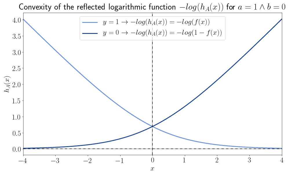
4.4. Error Function and Optimization

This implies that we can define an error function $Err(h_A, y)$ that has the form of $-log(h_A, y)$ . This function is then convex for all values of its input. Since the likelihood function is the one we use to learn the parameters of the model, its log-likelihood is the one we then use as an error function:

$Err(h_A, y) = -log(h_A(x))\ y - log(1-h_A(x))(1-y)$

We can rewrite the problem of optimization in terms of the minimization of this function over all the observed samples, as:

$J(A) = \frac{1}{n}\sum_{i=1}^{n}[-log(h_A(x))\ y - log(1-h_A(x))(1-y)]$

4.5. Convexity, Gradient Descent, and Log-Likelihood

We can now sum up the reasoning that we conducted in this article in a series of propositions that represent the theoretical inference that we’ve conducted:

The error function is the function through which we optimize the parameters of a machine learning model
This optimization takes place through algorithmic methods for learning
The method most commonly used for logistic regression is gradient descent
Gradient descent requires convex cost functions
Mean Squared Error, commonly used for linear regression models, isn’t convex for logistic regression
This is because the logistic function isn’t always convex
The logarithm of the likelihood function is however always convex

We, therefore, elect to use the log-likelihood function as a cost function for logistic regression. On it, in fact, we can apply gradient descent and solve the problem of optimization.

5. Conclusions

In this article, we studied the reasoning according to which we prefer to use logarithmic functions such as log-likelihood as cost functions for logistic regression.

We’ve first studied, in general terms, what characteristics we expect a cost function for parameter optimization to have. We’ve then seen what characteristics does the maximum likelihood function, in its basic form, possess.

Lastly, we studied the characteristics of the logarithmic version of that function. Because of its guaranteed convexity, we argued that it’s preferable to use that instead of the mean squared error.

Full Archive

About Baeldung

Core Concepts

Operating Systems

Artificial Intelligence

Graph Theory

Latex