Support Vector Machines (SVM) | Baeldung on Computer Science

1. Overview

In this tutorial, we’re going to study the theory and the mathematical foundation of support vector machines.

First, we’re going to discuss the problem of optimal decision boundaries for the linear separation of classes. Then, we’ll study how support vector machines guarantee the finding of these boundaries.

After discussing linear support vector machines, we’re also going to address the identification of non-linear decision boundaries. In doing so, we’ll enumerate the most common kernels for non-linear support vector machines.

At the end of this tutorial, we’ll be acquainted with the theoretical bases of support vector machines. We’ll know how to compute them over a dataset, and what kernels to apply if necessary.

2. The Problem of Identification of Decision Boundaries

2.1. Complexity as Separation

As anticipated in the introduction, we’re going to start this discussion on support vector machines (hereafter: SVM) by studying the problem of identification of decision boundaries in machine learning. In this manner, we’ll follow the tradition of our website to outline, in introductory articles on machine learning models, the type of prior knowledge that’s embedded in any given model.

One of the typical tasks in machine learning is the task of classification for supervised learning models. Many algorithms exist that perform these tasks, each of them having their own nuances. In other tutorials on our website, we’ve already studied logistic regression for classification, softmax in neural networks, and naive Bayesian classifiers, and we can refer to them for a refresh if we need it.

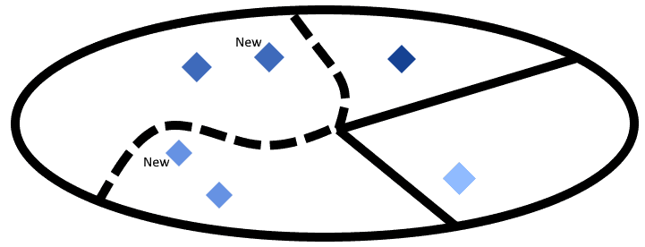
The idea behind classification in machine learning is that the world, or rather a vector space, can be separated into regions that possess different identifiable characteristics. In doing so, we presume that the world has a complexity that corresponds to distinct subsets of that world, not overlapping one another. The world can thus be divided into distinct regions, comprising distinct classes of things, each of them having their own elements:

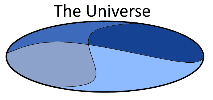
This is particularly important in the context of SVM, for reasons that we’ll see shortly.

2.2. Using the Territory as the Map

We could then ask ourselves how can we describe this world in terms of its categories, and find a comprehensive formal description that leaves no region untouched. In other words, we could ask ourselves how to create a map that allows us to identify the class affiliation of any points or observations contained in that world. We’re interested, of course, in the most simple summary that works for all points, or as many as possible.

One way to do so is to create an infinite set, list, or dictionary, comprising of all existing points in that world and their associated classification. This is done by sampling the whole world, point by point, and then composing a description that consists of the classes or categories that we observe at each location:

If we did so, we could come up with a map that consists of the list of categories or classes that we observe at each individual point. If we represent the classes with the numbers from 1 to 4, for example, we could define an infinite set that looks like this:

$\text{MAP}: \{(x_1 \mapsto 1); (x_2 \mapsto 3); (x_3 \mapsto 4) ; (x_4 \mapsto 2); ... \}$

If we imagine sampling the world to an arbitrary resolution, we would thus create a map that contains all points of that world, or as many as we want, and the classes associated with them.

This approach is perfectly legitimate but unlikely to take place in practice. The first reason is that it requires the possibility to sample the feature space to an arbitrarily high resolution. The second reason is that the map requires as much information as the whole world that it describes, making it redundant to then use the map rather than the world to which it points.

2.3. Understanding Complexity by Identifying Separation

We could, however, use a different approach based upon the prior knowledge that the regions in which our world is divided are not-overlapping:

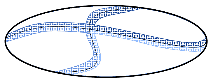
This approach would suggest using a subset of each region to define that same region. We could, in fact, explicitly identify only a subregion $S$ of each region $R$ , such that the subregion plus its complement corresponds to that region: $S + (R \ S) = R$ .

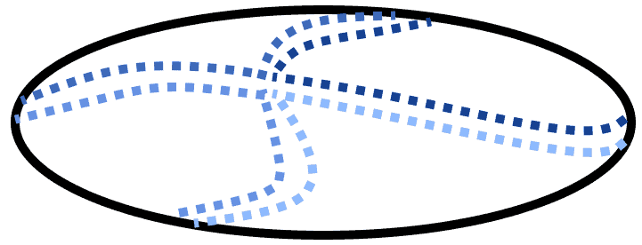
We could then explicitly list only the points contained in the subregion $S$ , as done before, and consider all other points in any complement subset $R \ S$ as belonging to the same class as the class of any elements in the closest subregion $S$ . This means that we would only do the sampling on a small subset of each region, and in particular on those subsets that border analogous subsets of other regions.

This method of summarizing is less complex than the previous one. This is because we’re explicitly enumerating only some of the points and their respective classes, not the whole region. The remaining class affiliations we extrapolate on the basis of a procedure, thus requiring less explicit information.

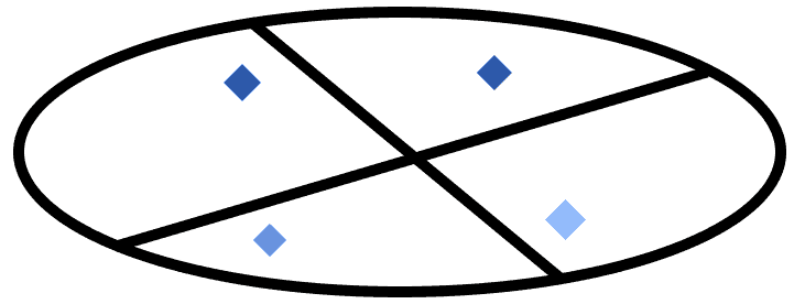
2.4. The Most Proximate but Different Observations

We could, however, do an even better job of summing up the complexity of this world. All we need to do is to consider that we don’t really need a whole subregion to individuate the boundary between classes, but just a few points. Specifically, the ones located closest to the boundary between regions; or rather, as close as we arbitrarily decide:

Now, the proximity of these points with one another will depend on the resolution of our sampling. A higher resolution would correspond here to points closer to one another, and to the boundaries within regions, and vice-versa. But regardless of the resolution, as long as we have at least one point in each region, we can always imagine that the boundaries are located somewhere between the closest points which belong to different classes:

The accuracy of the boundaries that we identify vis-à-vis the real complexity of the world may change greatly, according to the resolution of our sampling. But in any case, a boundary can be identified, which will be correct against at least some parts of the space.

2.5. Learning a More Accurate Representation

The process of identification of the borders can also be interpreted from a dynamic or online perspective. We can imagine that, once we identify a potential boundary as in the example above, we then receive new observations that falsify our prediction. In this case, we would simply shift the boundary that we had identified in order to accommodate the new observations:

Support vector machines work in this manner. By identifying first the closest observations that don’t belong to the same class, they then propose a decision boundary that gathers all observations of the same class inside one region. Only, they also select the possible decision boundary that maximizes the distance with the closest known observations, as we’ll see shortly.

3. The Mathematical Formulation of SVMs

3.1. Linear SVMs for Linearly Separable Problems

We can now move towards the mathematical formalization of the procedure that we’ve described above. If we have a dataset comprising of observations, these span a feature space $V = \mathbb{R}^{|x|}$ . Here, $|x|$ is the dimensionality of the vector comprising of the features for a given observation $x$ .

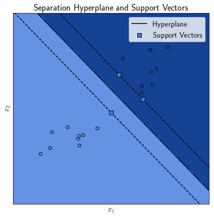
In this feature space $V$ , an SVM identifies the hyperplane that maximizes the distance that exists between itself and the closest two points or sets of points that belong to distinct categories. If one such hyperplane exists, we can say that the observations are linearly separable in the feature space $V$ :

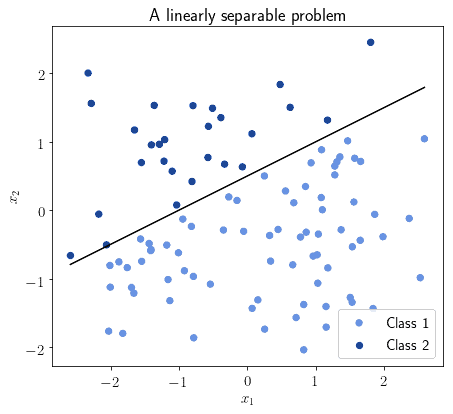
Not all problems, however, are linearly separable. Let’s keep in mind that for this section we’re only referring to those that are; see later for a discussion of non-linear SVMs.

3.2. Separation Hyperplane and Support Vectors

In this case, we can say that an SVM that identifies a hyperplane for a linearly separable problem is a linear SVM. We’re going to see in a second the formula for computing this hyperplane. Before we do that, let’s reason about what input this function needs to have.

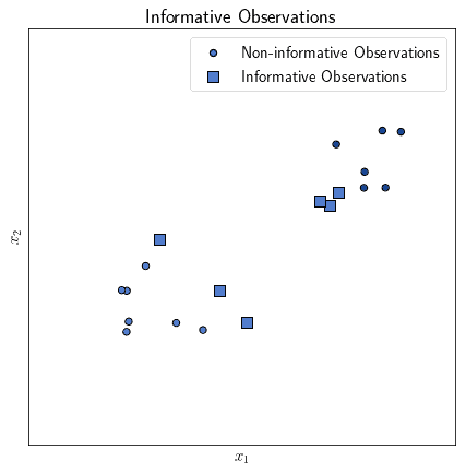
We can naively try to identify the separation hyperplane by looking at the whole collection of points or observations. This means that the input to any learning function we’d use would however have a significant number of largely uninformative features. As we discussed in the section on the identification of decision boundaries, above, the only informative observations we require are those located in closest proximity to the decision boundary:

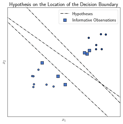
We don’t yet know where exactly the decision boundary is before we learn it, of course. We can, however, presume, under the hypothesis of linear separability, the following. If any pair of observations belong to two different classes, then the hyperplane lies somewhere between them:

These informative observations, or rather their feature vectors, support the identification of the decision boundary by the SVM. For this reason, we call the feature vectors located in proximity to observations of other classes “support vectors”. From this name, in turn, comes the name of “support vector machine”.

3.3. Identification of the Decision Boundary

Let’s now delve into the process of identification of this hyperplane for the separation of classes. A general formula for the description of a hyperplane $h_V$ in a vector space $V$ is:

$\overrightarrow{v} \cdot \overrightarrow{x} - b = 0$

where $v$ is the normal vector to this hyperplane. In case the term $b$ equals 0, the hyperplane is also a subspace of the original vector space, but this isn’t required.

We can reframe the problem of identifying the decision boundary, as a problem of identification of the normal vector $\overrightarrow{v}$ and the parameter $b$ . This identification must respect the constraint regarding the maximization of distance. In other words, the hyperplane must be the farthest to the two closest observations that belong to distinct classes.

We can call the decision function we’re learning as $y = f(x)$ . If the two classes are encoded by the values 1 and -1, such that $y_i = f(x_i) \to y_i = 1 \vee y_i = -1$ , we can then write the problem as:

$\text{min}(||\overrightarrow{v}||): y_i (\overrightarrow{v} x_i + b) \geq 1$

On one hand, the observations belonging to class $y = 1$ can be represented by an inequality $(\overrightarrow{v} x_i + b) \geq 1$ . Those belonging to the class $y = -1$ are represented instead by the inequality $(\overrightarrow{v} x_i + b) \leq -1$ . The two can thus be simplified as:

$[ (\overrightarrow{v} x_i + b) \geq y_i | y_i = 1 ] \vee [ (\overrightarrow{v} x_i + b) \leq y_i | y_i = -1 ] \leftrightarrow y_i (\overrightarrow{v} x_i + b) \geq 1$

This formula finally corresponds to the one whose term $\overrightarrow{v}$ we minimized in the previous expression. The hyperplane that we identify as a decision boundary is thus the one located halfway between the ones that act as limits for the two half-spaces, corresponding to the inequalities defined above:

4. Non-Linear SVMs

4.1. Non-Linear Decision Boundaries

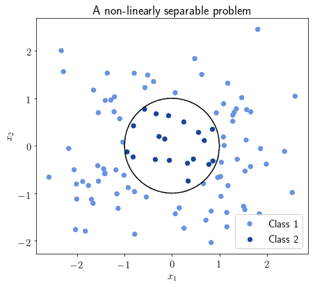
Some classes of problems aren’t however linearly separable. In this case, we say that there’s no hyperplane of the feature space that can be a decision boundary. A decision boundary can however still exist; it simply won’t be a hyperplane for $V$ :

Even though it won’t be a hyperplane of the feature space, it might still be a hyperplane in some transformed vector space. Let’s call this transformed space $W = \mathbb{R}^m$ . The dimensionality of $W$ is expected to be equal or higher to that of $V$ so that $|W| \geq |V|$ .

The task of identification of a decision boundary for non-linearly separable problems can thus be reframed in the following manner. First, we can find a mapping that projects the feature space $V$ to a vector space $W$ with transformed topology:

$f: V = \mathbb{R}^{|x|} \mapsto W = \mathbb{R}^m \leftrightarrow |x| \leq m$

We can then replace any dot products that we would compute between two feature vectors in the non-transformed vector space $V$ with that of the corresponding transformed space:

$x_i, x_j \in V: k(x_i \cdot x_j) = \chi_i \cdot \chi_j | \chi_i, \chi_j \in W \leftrightarrow \chi_i = f(x_i) \wedge \chi_j = f(x_j)$

There’s a function that replaces the dot product of two vectors in the original space with the transformed dot product, in terms of the non-transformed vectors. This function is called kernel $k$ of the SVM; the kernel is such that $k(x_i,x_j) = f(x_i) \cdot f(x_j)$ .

The hyperplane $h_W$ computed in the transformed vector space has a normal vector $\overrightarrow{\omega} = \sum \alpha y f(x)$ . This, in turn, allows us to compute it as $h_W = \omega \cdot \chi + \beta$ in the transformed space $W$ and with the transformed observations $\chi = f(x)$ .

We can then project back the hyperplane to the original vector space $V$ . The projection occurs by means of the inverse mapping $f^{-1}$ , as $h_V = f^{-1}(h_W)$ .

4.2. Non-Linear Kernels for SVMs

We can now enumerate the most common types of kernel functions used in non-linear SVMs. These correspond to as many transformations between the original feature space $V$ and the transformed $W$ . The most common kernels are:

The polynomial kernel of degree $p$ , $(x_i, x_j)^p$
The radial basis function kernel, $e^{-a||x_i - x_j||^{2}}$ , with $a>0$
The sigmoid $tanh(a \cdot x_i \cdot x_j + c)$

The choice of which specific kernel to use then depends on the problem we tackle. The determination is in any case based upon heuristics and has little theoretical value. In practice, the kernels are all tested in turn until we found one whose accuracy is satisfactory.

5. Conclusions

In this tutorial, we studied the theoretical foundation of support vector machines and described them mathematically.

We first started by discussing, in general, the problem of identification of decision boundaries for classification. In this context, we noticed how the observations in the proximity of the decision boundary carry the most information.

We then discussed the issue of identifying a hyperplane for the linear separation of classes. We also named “support vectors” the most informative features in a class, those located in proximity to the decision hyperplane.

Lastly, we discussed the problem of identification of a decision boundary for problems that aren’t linearly separable. In relation to this, we studied how to transform the original vector space into one where a solution exists. We also discussed the usage of kernel functions and defined the most common ones used in non-linear SVMs.

Full Archive

About Baeldung

Core Concepts

Operating Systems

Artificial Intelligence

Graph Theory

Latex