

Learn through the super-clean Baeldung Pro experience:
>> Membership and Baeldung Pro.
No ads, dark-mode and 6 months free of IntelliJ Idea Ultimate to start with.
Last updated: March 26, 2025
Learn through the super-clean Baeldung Pro experience:
>> Membership and Baeldung Pro.
No ads, dark-mode and 6 months free of IntelliJ Idea Ultimate to start with.
In this tutorial, we’ll study what are learning curves and why they are necessary during the training process of a machine learning model.
We’ll also discover different types of curves, what they are used for, and how they should be interpreted to make the most out of the learning process.
By the end of the article, we’ll have the theoretical and practical knowledge required to avoid common problems in real-life machine learning training. Ready? Let’s begin!
Contrary to what people often think, machine learning is far from being fully automated. It requires lots of “babysitting”; monitoring, data preparation, and experimentation, especially if it’s a new project. In all that process, learning curves play a fundamental role.
A learning curve is just a plot showing the progress over the experience of a specific metric related to learning during the training of a machine learning model. They are just a mathematical representation of the learning process.
According to this, we’ll have a measure of time or progress in the x-axis and a measure of error or performance in the y-axis.
We use these charts to monitor the evolution of our model during learning so we can diagnose problems and optimize the prediction performance.
The most popular example of a learning curve is loss over time. Loss (or cost) measures our model error, or “how bad our model is doing”. So, for now, the lower our loss becomes, the better our model performance will be.
In the picture below, we can see the expected behavior of the learning process:
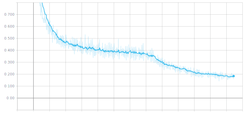
Despite the fact it has slight ups and downs, in the long term, the loss decreases over time, so the model is learning.
Other examples of very popular learning curves are accuracy, precision, and recall. All of these capture model performance, so the higher they are, the better our model becomes.
See below an example of a typical accuracy curve over time:
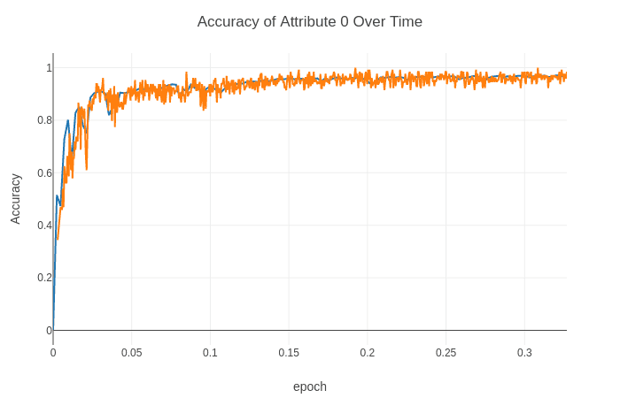
The model performance is growing over time, which means the model is improving with experience (it’s learning).
We also see it grows at the beginning, but over time it reaches a plateau, meaning it’s not able to learn anymore.
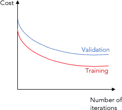
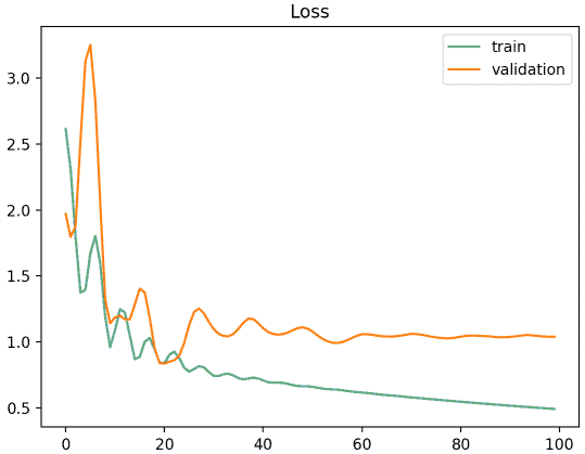
One of the most widely used metrics combinations is training loss + validation loss over time.
The training loss indicates how well the model is fitting the training data, while the validation loss indicates how well the model fits new data.
We will see this combination later on, but for now, see below a typical plot showing both metrics:
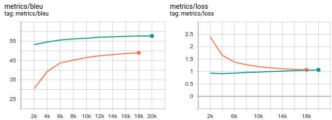
Another common practice is to have multiple metrics in the same chart as well as those metrics for different models.
We often see these two types of learning curves appearing in charts:
Below you can see an example in Machine Translation showing BLEU (a performance score) together with the loss (optimization score) for two different models (orange and green):
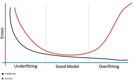
We can detect issues in the behavior of a model by watching the evolution of a learning curve.
Next, we’ll see each of the different scenarios we can find for model behavior detection:
Let’s quickly review what these concepts are:
We can see they are closely tied, as the more biased a model is, the more it underfits the data.
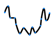
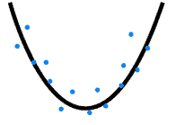
Let’s imagine our data are the blue dots below, and we want to come up with a linear model for regression purposes:
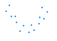
Suppose we’re very lazy machine learning practitioners and we propose this line as a model:
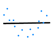
Clearly, a straight line like that doesn’t represent the pattern of our dots. It lacks some complexity to describe the nature of the given data. We can see how the biased model doesn’t take into account relevant information, which leads to underfitting.
It’s doing a terrible job with the training data already, so what would be the performance for a new example?
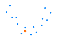
It’s pretty obvious it performs as poorly with the new example as it does with the training data:
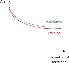
Now, how can we use learning curves to detect our model is underfitting? See an example showing validation and training cost (loss) curves:
Let’s briefly review these two concepts:
These are also directly related concepts: The higher the variance of a model, the more it overfits the training data.
Let’s take the same example as before, where we wanted a linear model to approximate these blue dots:
Now, on the other extreme, let’s imagine we’re very perfectionist machine learning practitioners and we propose a linear model that perfectly explains our data like this:
Well, we understand intuitively that this line is not what we wanted, either. Indeed, it fits the data, but it doesn’t represent the real pattern in it.
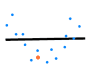
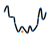
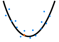
When a new example appears, it will struggle to model it. See a new example (in orange):
Using the overfitted model, it won’t predict well enough the new example:
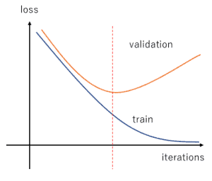
How could we use learning curves to detect a model is overfitting? We’ll need both the validation and training loss curves:
The solution to the bias/variance problem is to find a sweet spot between them.
In the example given above:
a good linear model for the data would be a line like this:
So, when a new example appears:
We will make a better prediction:
We can use the validation and training loss curves to find the right bias/variance tradeoff:
A representative dataset reflects proportionally statistical characteristics in another dataset from the same domain.
We could find the training dataset is not representative in relation to the validation dataset and vice-versa.
This happens when the data available during training is not enough to capture the model, relative to the validation dataset.
We can spot this issue by showing one loss curve for training and another for validation:
The train and validation curves are improving, but there’s a big gap between them, which means they operate like datasets from different distributions.
This happens when the validation dataset does not provide enough information to evaluate the ability of the model to generalize.
The first scenario is:
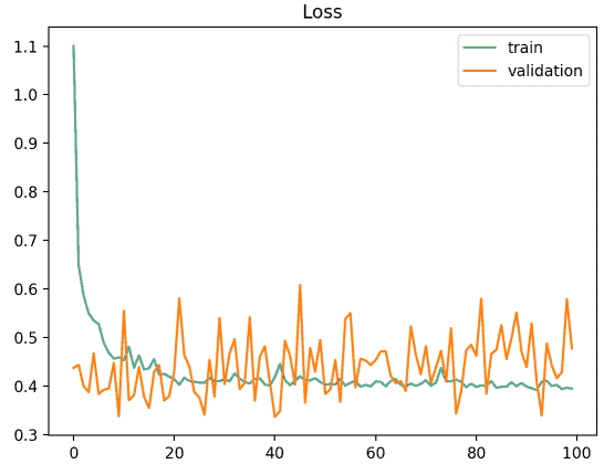
As we can see, the training curve looks ok, but the validation function moves noisily around the training curve.
It could be the case that validation data is scarce and not very representative of the training data, so the model struggles to model these examples.
The second scenario is:
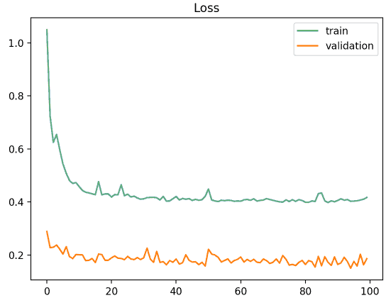
Here we find the validation loss is much better than the training one, which reflects the validation dataset is easier to predict than the training dataset.
An explanation could be the validation data is scarce but widely represented by the training dataset, so the model performs extremely well on these few examples.
Anyway, this means the validation dataset does not represent the training dataset, so there is a problem with representativeness.
In this tutorial, we reviewed some basic concepts required to understand the concepts behind learning curves and how to use them.
Next, we learned how to interpret learning curves and the way they can be used to avoid common learning problems such as underfitting, overfitting, or unrepresentativeness.