Yes, we're now running our only Summer Sale. All Courses are 30% off until 20th July, 2026:
What Is the Difference Between Gradient Descent and Gradient Ascent?
Last updated: March 26, 2025

Learn through the super-clean Baeldung Pro experience:
>> Membership and Baeldung Pro.
No ads, dark-mode and 6 months free of IntelliJ Idea Ultimate to start with.
1. Overview
In this tutorial, we’ll study the difference between gradient descent and gradient ascent.
At the end of this article, we’ll be familiar with the difference between the two and know how to convert from one to the other.
2. The Gradient in General
The gradient of a continuous function  is defined as the vector that contains the partial derivatives
  computed at that point
  . The gradient is finite and defined if and only if all partial derivatives are also defined and finite. With formal notation, we indicate the gradient as:
![\nabla f(x) = [\frac{\delta{f}}{\delta{x_1}}(p), \frac{\delta{f}}{\delta{x_2}}(p), ... , \frac{\delta{f}}{\delta{x_{|x|}}}(p)]^T](/wp-content/ql-cache/quicklatex.com-133a31967b684d56f788e2ceaf4d4a89_l3.svg "Rendered by QuickLaTeX.com")
When using the gradient for optimization, we can either conduct gradient descent or gradient ascent. Let’s now see the difference between the two.
3. Gradient Descent
Gradient descent is an iterative process through which we optimize the parameters of a machine learning model. It’s particularly used in neural networks, but also in logistic regression and support vector machines.
It’s the most typical method for iterative minimization of a cost function. Its major limitation, though, consists of its guaranteed convergence to a local, not necessarily global, minimum:
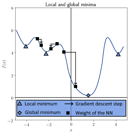
A hyperparameter  , also called the learning rate, allows the fine-tuning of the process of descent. In particular, with an appropriate choice of , we can escape the convergence to a local minimum, and descend towards a global minimum instead.
The gradient is calculated with respect to a vector of parameters for the model, typically the weights  . In neural networks, the process of applying gradient descent to the weight matrix takes the name of the backpropagation of the error.
Backpropagation uses the sign of the gradient to determine whether the weights should increase or decrease. The sign of the gradient allows us to decide the direction of the closest minimum to the cost function. For a given parameter , we iteratively optimize the vector by computing:

And this is the graphical representation:
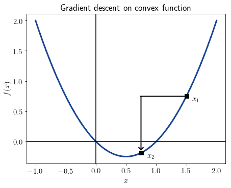
We can read the formula above like this. At step  , the weights of the neural network are all modified by the product of the hyperparameter times the gradient of the cost function, computed with those weights. If the gradient is positive, then we decrease the weights; and conversely, if the gradient is negative, then we increase them.
4. Gradient Ascent
Gradient ascent works in the same manner as gradient descent, with one difference. The task it fulfills isn’t minimization, but rather maximization of some function. The reason for the difference is that, at times, we may want to reach the maximum, not the minimum of some function; this is the case, for instance, if we’re maximizing the distance between separation hyperplanes and observations.
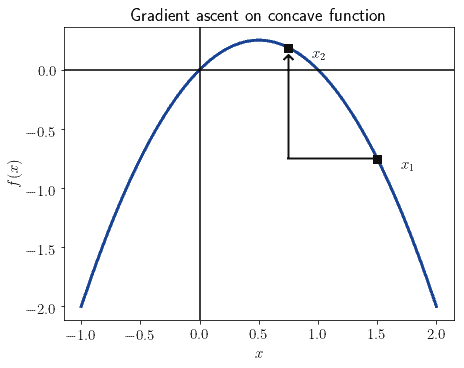
For this reason, the formula that describes gradient ascent is similar to the one for gradient descent. Only, with a flipped sign:

If gradient descent indicates an iterative movement towards the closest minimum, gradient ascent, conversely, indicates a movement towards the nearest maximum. In this sense, for any function on which we apply gradient descent, there is a symmetric function  on which we can apply gradient ascent.
This means also that a problem tackled through gradient descent also has solutions that we can find through gradient ascent, if only we reflect it upon the axis of the independent variable. This image shows the same function of the previous graph, but reflected along the  axis:
axis:
In our article on the cost function for logistic regression, we studied the usage of the log-likelihood and its relation to convexity. If we use a positive log-likelihood, then the objective function is concave and we must use gradient ascent. Conversely, if we use negative log-likelihood, as is common practice, we should instead use gradient descent.
This is because gradient descent works on convex objective functions, while gradient ascent requires concave functions.
5. Gradient Descent or Gradient Ascent?
We can now sum-up the considerations made above:
- The gradient is the vector containing all partial derivatives of a function in a point
- We can apply gradient descent on a convex function, and gradient ascent on a concave function
- Gradient descent finds the nearest minimum of a function, gradient ascent the nearest maximum
- We can use either form of optimization for the same problem if we can flip the objective function
With this said, gradient descent is more common in practice than gradient ascent.
6. Conclusions
In this tutorial, we studied the concept of gradient, and learned the distinction between gradient descent and gradient ascent.