

Yes, we're now running our only Summer Sale. All Courses are 30% off until 20th July, 2026:
Traveling Salesman Problem – Dynamic Programming Approach
Last updated: March 18, 2024
Learn in
Learn through the super-clean Baeldung Pro experience:
>> Membership and Baeldung Pro.
No ads, dark-mode and 6 months free of IntelliJ Idea Ultimate to start with.
1. Overview
The Travelling Salesman Problem (TSP) is a very well known problem in theoretical computer science and operations research. The standard version of TSP is a hard problem to solve and belongs to the NP-Hard class.
In this tutorial, we’ll discuss a dynamic approach for solving TSP. Furthermore, we’ll also present the time complexity analysis of the dynamic approach.
2. Introduction to TSP
In the TSP, given a set of cities and the distance between each pair of cities, a salesman needs to choose the shortest path to visit every city exactly once and return to the city from where he started.
Let’s take an example to understand the TSP in more detail:
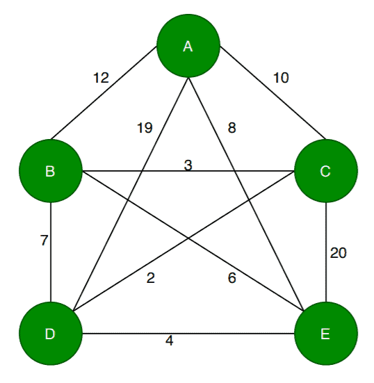
Here, the nodes represent cities, and the values in each edge denote the distance between one city to another. Let’s assume a salesman starts the journey from the city  . According to TSP, the salesman needs to travel all the cities exactly once and get back to the city by choosing the shortest path. Here the shortest path means the sum of the distance between each city travelled by the salesman, and it should be less than any other path.
With only  cities, the problem already looks quite complex. As the graph in the example is a complete graph, from each city, the salesman can reach any other cities in the graph. From each city, the salesman needs to choose a route so that he doesn’t have to revisit any city, and the total distance travelled should be minimum.
How to find out such a path? Let’s discuss an algorithm to solve the TSP problem.
3. Dynamic Programming Approach for Solving TSP
Let’s first see the pseudocode of the dynamic approach of TSP, then we’ll discuss the steps in detail:
algorithm DynamicApproachForTSP(s, N, dist):
    // INPUT
    //    sp = starting point
    //    N = a subset of input cities
    //    dist = function to compute distance among the cities
    // OUTPUT
    //    Cost = the cost of the TSP solution
    visited <- data structure to track visited cities
    for x in N:
        visited[x] <- 0
    Cost <- a matrix initialized with zero values

    return TSP(N, sp)

    function TSP(N, s):
        visited[s] <- 1

        if |N| = 2 and k != s:
            Cost[N, k] <- dist(s, k)
            return Cost
        else:
            for j in N:
                for i in N and Visited[i] = 0:
                    if j != i and j != s:
                        Cost[N, j] <- min(TSP(N - {i}, j) + dist(j, i))
                        visited[j] <- 1

        return Cost
In this algorithm, we take a subset  of the required cities needs to be visited, distance among the cities
  and starting city
  as inputs. Each city is identified by unique city id like
  .
.
Initially, all cities are unvisited, and the visit starts from the city . We assume that the initial travelling cost is equal to  . Next, the TSP distance value is calculated based on a recursive function. If the number of cities in the subset is two, then the recursive function returns their distance as a base case.
On the other hand, if the number of cities is greater than  , then we’ll calculate the distance from the current city to the nearest city, and the minimum distance among the remaining cities is calculated recursively.
Finally, the algorithm returns the minimum distance as a TSP solution.
Here we use a dynamic approach to calculate the cost function  . Using recursive calls, we calculate the cost function for each subset of the original problem.
4. Time Complexity Analysis
In the dynamic algorithm for TSP, the number of possible subsets can be at most  . Each subset can be solved in
  times. Therefore, the time complexity of this algorithm would be
  .
.
5. Conclusion
TSP is a popular NP-Hard problem, but depending on the size of the input cities, it is possible to find an optimal or a near-optimal solution using various algorithms.
In this tutorial, we’ve discussed a dynamic programming approach for solving TSP. We also presented the time complexity of the given algorithm.