Minimum Spanning Tree vs Shortest Path Tree

1. Introduction

In this tutorial, we’ll focus on two problems: Minimal Spanning Tree and Shortest Path Tree. We can solve both problems with greedy algorithms that have a similar structure.

2. Spanning Tree

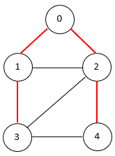
A spanning tree of an undirected graph G is a connected subgraph that covers all the graph nodes with the minimum possible number of edges. In general, a graph may have more than one spanning tree.

The following figure shows a graph with a spanning tree. The edges of the spanning tree are in red:

3. Minimum Spanning Tree 

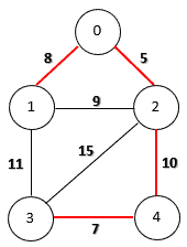
If the graph is edge-weighted, we can define the weight of a spanning tree as the sum of the weights of all its edges. A minimum spanning tree is a spanning tree whose weight is the smallest among all possible spanning trees. 

The following figure shows a minimum spanning tree on an edge-weighted graph:

We can solve this problem with several algorithms including Prim’s, Kruskal’s, and Boruvka’s.

Let’s introduce Prim’s algorithm since it has a similar structure with the solution to the shortest path tree problem:

algorithm PrimsAlgorithmForMST:
    // INPUT
    //    G = a graph with weighted edges
    // OUTPUT
    //    Returns the minimum spanning tree

    Initialize a node set S1 with an arbitrary node u from G
    Put all the other nodes in G into a node set S2
    Initialize an empty edge set T to store minimum spanning tree edges
    Initialize an edge set E to store edges that have one end node in S1 and another end node in S2
    Insert all edges {{u, v} | v in S2} into E
    while S2 is not empty:
        Select an edge {u, v | u in S1, v in S2} from E that has the minimum weight
        Add {u, v} to T
        Remove {u, v} from E
        Remove v from S2 and add it to S1
        Insert all edges {v, w | w in S2} into E
    return T

Visually, let’s run Prim’s algorithm for a minimum spanning tree on our sample graph step-by-step:

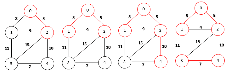
The time complexity of Prim’s algorithm depends on the data structures used for the graph.

For example, if we use the adjacency list to represent a graph and store the edges in a priority queue, the overall time complexity is O(E log V), where V is the number of nodes in the graph and E is the number of edges. Also, the overall time complexity is O(V²), if we use the adjacency matrix to represent a graph.

4. Shortest Path Tree

In the shortest path tree problem, we start with a source node s.

For any other node v in graph G, the shortest path between s and v is a path such that the total weight of the edges along this path is minimized. Therefore, the objective of the shortest path tree problem is to find a spanning tree such that the path from the source node s to any other node v is the shortest one in G.

We can solve this problem with Dijkstra’s algorithm:

algorithm DijkstrasAlgorithmForShortestPathTree:
    // INPUT
    //    G = a graph with weighted edges
    //    s = the source node
    // OUTPUT
    //    A shortest path tree of G rooted at s

    Initialize a node set S1 with s
    Assign a distance value 0 to node s: Dist(s) <- 0
    Put all the other nodes in G into a node set S2
    Initialize an empty edge set T to store shortest path tree edges
    Initialize an edge set E to store edges that have one end node in S1 and another end node in S2
    Add all edges {u, v | v in S2} into E
    while S2 is not empty:
        Select an edge {u, v | u in S1, v in S2} from E that has the minimum Dist(u) + weight(u, v)
        Add {u, v} to T
        Remove {u, v} from E
        Remove v from S2 and add it to S1
        Dist(v) <- Dist(u) + weight(u, v)
        Add all edges {v, w | w in S2} into E
    return T

Dijkstra’s algorithm has a similar structure to Prim’s algorithm. However, they have different selection criteria.

In Prim’s algorithm, we select the node that has the smallest weight. However, in Dijkstra’s algorithm, we select the node that has the shortest path weight from the source node. Therefore, the resulting spanning tree can be different for the same graph.

Let’s visually run Dijkstra’s algorithm for source node number 0 on our sample graph step-by-step:

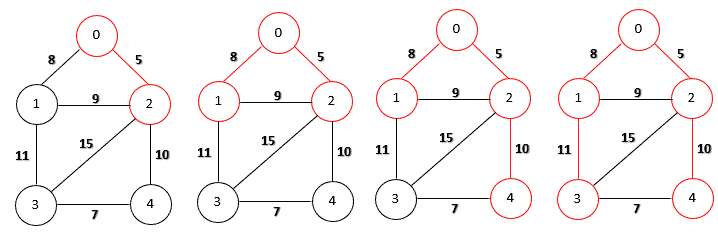
The shortest path between node 0 and node 3 is along the path 0->1->3. However, the edge between node 1 and node 3 is not in the minimum spanning tree. Therefore, the generated shortest-path tree is different from the minimum spanning tree.

Similar to Prim’s algorithm, the time complexity also depends on the data structures used for the graph. The overall time complexity is O(V²) if we use the adjacency matrix to represent a graph. Also, if we use the adjacency list to represent a graph and store the edges in a priority queue, the overall time complexity is O(E log V).

5. Conclusion

In this tutorial, we discussed two similar problems: Minimum Spanning Tree and Shortest-Path Tree. Also, we compared the difference between Prim’s and Dijkstra’s algorithms.

Detailed implementations are available in our articles about Prim’s and Dijkstra’s algorithms, respectively.