

Learn through the super-clean Baeldung Pro experience:
>> Membership and Baeldung Pro.
No ads, dark-mode and 6 months free of IntelliJ Idea Ultimate to start with.
Learn through the super-clean Baeldung Pro experience:
>> Membership and Baeldung Pro.
No ads, dark-mode and 6 months free of IntelliJ Idea Ultimate to start with.
Genetic algorithms and neural networks are completely different concepts and are used to solve different problems. In this article, first, we’ll start with a short general introduction to genetic algorithms and neural networks. Then, we’ll outline some guidelines for when we should use each of these techniques using a couple of examples. Finally, we’ll conclude the article by making a high-level comparison between these two techniques.
Along the way, we’ll also cover some interesting facts about these algorithms that make them different from other general algorithms.
Let’s start by discussing some of the basics of the genetic algorithm and neural network.
The genetic algorithm is search heuristic which is inspired by Darwin’s theory of natural evolution. It reflects the process of the selection of the fittest element naturally.
A genetic algorithm starts with an initial population. From the initial population, this algorithm produces a new population using selection, crossover, and mutation steps:
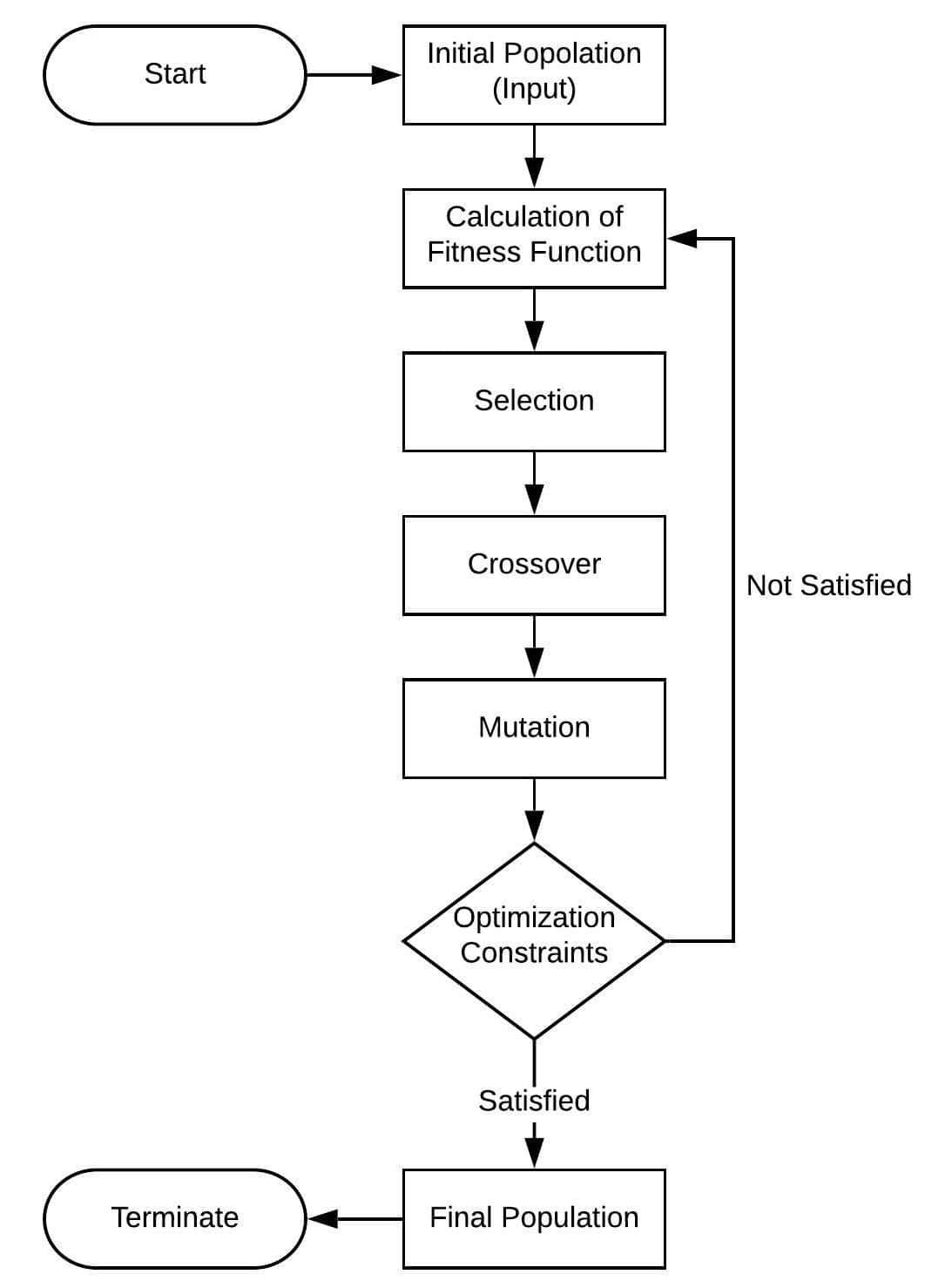
The algorithm takes the initial population as input and chooses a fitness function. The fitness function helps the algorithm to generate an optimal or near-optimal solution. The algorithm continues and evolves the population through selection, crossover, and mutation operations. It generates several populations until it satisfies the optimization constraints.
On the other hand, a neural network consists of a series of algorithms that endeavor to determine and identify patterns. It works similarly to how a human brain’s neural network works. In algorithms, a neural network refers to a network of neurons, where a neuron is a mathematical function used to collect as well as to classify data from a given model.
A neural network can contain weights and many hidden layers:
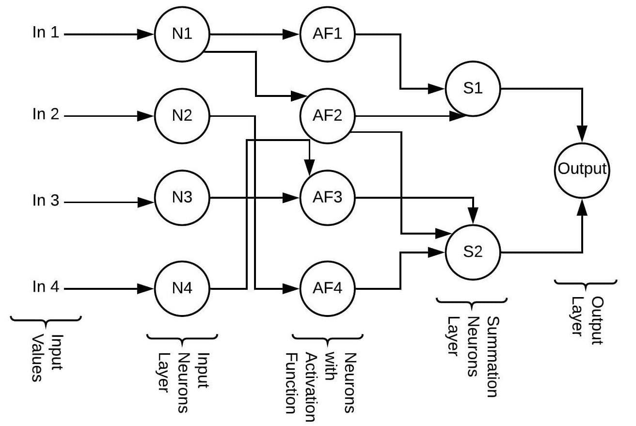
The inputs from the users form the input neuron layer in a neural network. The activation function layer determines the output. Depending upon the problem, it can have more than one activation function layer. The summation layer sums up the output generated by the activation function layer and then displays it in the output layer section.
Biological systems are known to be highly-optimized and adaptive systems. The intention behind the genetic algorithm is to develop an adaptive and artificially intelligent system.
Genetic algorithms are generally used for search-based optimization problems, which are difficult and time-intensive to solve by other general algorithms. Optimization problems refer to either maximization or minimization of the objective function. The genetic algorithm aims to find the optimal or near-optimal solution to the optimization problem.
A neural network is a mathematical model that is capable of solving and modeling complex data patterns and prediction problems. Neural network algorithms are developed by replicating and using the processing of the brain as a basic unit. As it has the capability of mimicking the functionality and operation of the human brain, it can do anything that a human can do.
Neural networks have many applications:
Now let’s start to dig into more details and try to understand when a genetic algorithm is a good choice for a given problem.
A genetic algorithm is a search-based optimization method. Let’s assume we have a large set of discrete state-space of good solutions, and the only available solution is to evaluate all the combinations (brute-force method). In this case, a genetic algorithm can give a reasonably good solution, but the optimal solution is not guaranteed.
There are many NP-Hard problems and time-intensive problems in the computer science field that are extremely difficult to solve. For example, let’s consider the traveling salesperson problem (TSP). One of the real-life applications of the TSP is finding the shortest path between two cities. Now suppose a person is using a GPS while driving to find the shortest path from one city to another. Delay in the GPS to fetch an optimal route is, of course, not acceptable. In such cases, a genetic algorithm is a good choice to get a fast and fairly accurate solution.
Traditional calculus methods work well in the case of a single-peaked objective function, where it starts with a random point, moves towards the gradient, and stops as soon as it reaches the peak point. But in real life, problems like landscapes consist of many peaks and valleys. In such cases, the traditional calculus method might get stuck on the local maxima. A genetic algorithm in such cases is capable of finding the global maxima.
Let’s examine the cases when neural networks can be an efficient choice over genetic algorithms.
When there is a function approximation problem with continuous data, a neural network is the best to use.
Suppose we have a million images stored on a hard disk, and out of these images, we have to decide which one contains the image of a dog and which one contains the image of a cat. This is an example of a classification problem. This task can be performed efficiently by a neural network.
Finally, consider that we have a dataset containing the price and size of houses in a specific city. Given the size details of a house, the task is to predict the price. This is an example of a linear regression problem. In this case, using a neural network can give a good price prediction for each house.
In this section, we’ll go through a couple of example problems where we’ll apply a genetic algorithm and neural network.
Let’s talk about the MAXONE problem and see how we can use a genetic algorithm to solve it.
Suppose that we have some string of binary digits (string of 0’s and 1’s) and we want to maximize the number of 1’s in the binary string. Let’s assume that the initial population has N random strings of length L, and F denotes the fitness function. In the MAXONE problem, F is the number of 1’s present in the population.
algorithm MAXONE(initialPopulation, X):
    // INPUT
    //    initialPopulation = Initial population of binary strings
    //    X = expected number of 1's
    // OUTPUT
    //    Final population with the number of 1's in the population maximized

    while true:
        fitness = X:
            // Output Accepted
            print("Final Fitness:", fitness)
            break
        selectedPopulation <- Selection(initialPopulation)
        crossedOverPopulation <- Crossover(selectedPopulation)
        mutatedPopulation <- Mutation(crossedOverPopulation)
        initialPopulation <- mutatedPopulation
Here, the CountOne() function counts the number of 1’s in the initial population. X denotes any integer number of 1’s that is expected from this algorithm. The initial population evolves through selection, mutation, and crossover, and the algorithm calculates the fitness function again. If it satisfies the given constraints (the value of X), then the population is accepted, otherwise, it repeats the selection operation.
We are taking N=4 and L=4. Here is the randomly generated initial population:
M1 = 1011 F(M1) = 3
M2 = 0010 F(M2) = 1
M3 = 1010 F(M3) = 2
M4 = 0000 F(M4) = 0
As given in the above example, the total number of 1’s in the initial population is 6. The genetic algorithm aims to produce the new population with a greater number of 1’s by using selection, crossover, and mutation.
In selection, the strings with good fitness scores are preferred over the other strings to generate the new population with a higher number of 1’s. Suppose after the application of selection, we get the following population:
M1 = 1011 (M1)
M2 = 1010(M3)
M3 = 0010(M2)
M4 = 1011(M1)
Now, the reason to change M4 is that the fitness score of M4 is zero. So, our selection operation gives preference to the string M1 as it contains the greatest number of 1’s compared to the other strings in the initial population.
Now, let’s apply the crossover operation. In crossover, two strings are selected, and a random portion of both strings are exchanged to generate a new string. We are randomly choosing M4 and M3 for crossover. M1 and M2 will be unchanged after crossover:
The bits in red are exchanged between M3 and M4 during the crossover operation.
Now, let’s proceed to the mutation operation. In mutation, the idea is to change some existing bit or to introduce some bits in the string to maintain diversity:
The colored bits are changed during the mutation process. Now, it’s time to calculate the fitness function again:
F(M1) = 2
F(M2) = 4
F(M3) = 3
F(M4) = 3
So, the value of the fitness function in the new population is 12. Out of 16 bits, we now have 12 bits corresponding to 1. We started with the initial population where the number of 1’s in the population was 6. So, the new population has improved from the previous population.
The algorithm will continue iterating. The user can give some conditions for termination. For example, we can specify that whenever the fitness function equals 14, we want this algorithm to terminate.
In this section, we are going to create a very simple neural network to verify an AND table. The neural network will have an input layer and an output layer. Here, the edges contain weight:
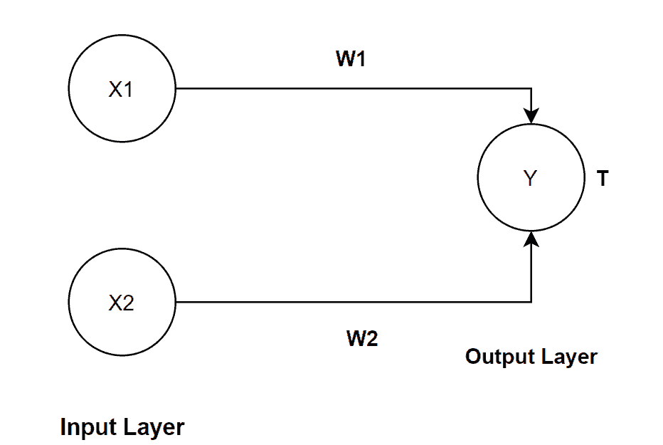
With this simple neural network, let’s explore how we can verify the AND gate. We are considering a two-input AND gate here.
The basic idea is that every node has a threshold value T. If the incoming signal is greater than the threshold value of the node, then the input values are not accepted (Generate 0). For the sake of simplicity, we’ll set the values for weights and thresholds manually for this example. The algorithm calculates the incoming signal for each node and then performs a checking step with the threshold value of the output node:
algorithm ANDGateVerification(Input values(X1, X2), Weights of the nodes(W1, W2)):
    // INPUT
    //    Input values(X1, X2) = Input values for the AND gate
    //    (W1, W2) = Weights of the neural network nodes
    // OUTPUT
    //    0 or 1 based on the AND operation result

    IncomingSignal <- X1*W1 + X2*W2
    if IncomingSignal > T:
        Generate output 1
    else:
        Generate output 0
        return
There are various ways to calculate weights and threshold values. In this example, we’ll use our prespecified values.
Weight of node X1 is W1(X1) = 1.5
Weight of node X2 is W2(X2) = 1.5
Threshold value of node Y is T(Y) = 2
First Input: X1 = 0, X2 = 0


Second Input: X1 = 0, X2 = 1


Third Input: X1 = 1, X2 = 0

Forth Input: X1 = 1, X2 = 1


Hence, with the help of this neural network algorithm, we successfully verified an AND table in this example.
We’ve discussed a lot regarding genetic algorithms and neural networks. Now, it’s time to put all the points that we have already discussed into a high-level comparison between the two techniques.
First of all, a genetic algorithms are search-based optimization algorithms used to find optimal or near-optimal solutions for search problems and optimization problems. Neural networks, on the other hand, are mathematical models that map between complex inputs and outputs. They can classify elements that are not previously known.
Genetic algorithms usually perform well on discrete data, whereas neural networks usually perform efficiently on continuous data.
Genetic algorithms can fetch new patterns, while neural networks use training data to classify a network.
A genetic algorithm doesn’t always require derivative information to solve a problem.
Genetic algorithms calculate the fitness function repeatedly to get a good solution. That’s why it takes a good amount of time to compute a reasonable solution. Neural networks, in general, take much less time for the classification of new input.
In this tutorial, we’ve discussed genetic algorithms and neural networks. We started with an introduction and motivation, and then we noted some general cases and guidelines for using the two techniques.
Furthermore, we have given some example problems and a high-level comparison between the two techniques to give the reader a better understanding.