Logistic Regression in Java
Last updated: May 20, 2025

Mocking is an essential part of unit testing, and the Mockito library makes it easy to write clean and intuitive unit tests for your Java code.
Get started with mocking and improve your application tests using our Mockito guide:
Handling concurrency in an application can be a tricky process with many potential pitfalls. A solid grasp of the fundamentals will go a long way to help minimize these issues.
Get started with understanding multi-threaded applications with our Java Concurrency guide:
Spring 5 added support for reactive programming with the Spring WebFlux module, which has been improved upon ever since. Get started with the Reactor project basics and reactive programming in Spring Boot:
Since its introduction in Java 8, the Stream API has become a staple of Java development. The basic operations like iterating, filtering, mapping sequences of elements are deceptively simple to use.
But these can also be overused and fall into some common pitfalls.
To get a better understanding on how Streams work and how to combine them with other language features, check out our guide to Java Streams:
Explore Spring Boot 3 and Spring 6 in-depth through building a full REST API with the framework:
Yes, Spring Security can be complex, from the more advanced functionality within the Core to the deep OAuth support in the framework.
I built the security material as two full courses - Core and OAuth, to get practical with these more complex scenarios. We explore when and how to use each feature and code through it on the backing project.
You can explore the course here:
Spring Data JPA is a great way to handle the complexity of JPA with the powerful simplicity of Spring Boot.
Get started with Spring Data JPA through the guided reference course:
Refactor Java code safely — and automatically — with OpenRewrite.
Refactoring big codebases by hand is slow, risky, and easy to put off. That’s where OpenRewrite comes in. The open-source framework for large-scale, automated code transformations helps teams modernize safely and consistently.
Each month, the creators and maintainers of OpenRewrite at Moderne run live, hands-on training sessions — one for newcomers and one for experienced users. You’ll see how recipes work, how to apply them across projects, and how to modernize code with confidence.
Join the next session, bring your questions, and learn how to automate the kind of work that usually eats your sprint time.
Yes, we're now running our only Summer Sale. All Courses are 30% off until 20th July, 2026:
Yes, we're now running our only Summer Sale. All Courses are 30% off until 20th July, 2026:
1. Introduction
Logistic regression is an important instrument in machine learning (ML) practitioner toolbox.
In this tutorial, we’ll explore the main idea behind logistic regression.
First, let’s start with a brief overview of ML paradigms and algorithms.
2. Overview
ML allows us to solve problems that we can formulate in human-friendly terms. However, this fact may represent a challenge for us software developers. We’ve accustomed ourselves to address the problems that we can formulate in computer-friendly terms. For example, as human beings, we can easily detect the objects on a photo or establish the mood of a phrase. How we could formulate such a problem for a computer?
In order to come up with a solution, in ML there is a special stage called training. During this stage, we feed the input data to our algorithm so that it tries to come up with an optimal set of parameters (the so-called weights). The more input data we may feed to the algorithm, the more precise predictions we may expect from it.
Training is a part of an iterative ML workflow:
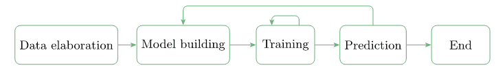
We start with acquiring data. Often, the data comes from different sources. Therefore, we have to make it be of the same format. We should control as well that the data set fairly represents the domain of study. If the model has never been trained on red apples, it can hardly predict it.
Next, we should build a model that’ll consume the data and will be able to make predictions. In ML, there are no pre-defined models that work well in all situations.
When searching for the correct model, it might easily happen that we build a model, train it, see its predictions and discard the model because we’re not happy with the predictions it makes. In this case, we should step back and build another model and repeat the process again.
3. ML Paradigms
In ML, based on what kind of input data we have at our disposal, we may single out three main paradigms:
- supervised learning (image classification, object recognition, sentiment analysis)
- unsupervised learning (anomaly detection)
- reinforcement learning (game strategies)
The case that we’re going to describe in this tutorial belongs to supervised learning.
4. ML Toolbox
In ML, there is a set of tools that we can apply when building a model. Let’s mention some of them:
- Linear regression
- Logistic regression
- Neural networks
- Support Vector Machine
- k-Nearest Neighbours
We may combine several tools when building a model that has high predictiveness. In fact, for this tutorial, our model will use logistic regression and neural networks.
5. ML Libraries
Even though Java is not the most popular language for prototyping ML models, it has a reputation as a reliable tool for creating robust software in many areas including ML. Therefore, we may find ML libraries written in Java.
In this context, we may mention the de-facto standard library Tensorflow which has a Java version as well. Another worth mentioning is a deep learning library called Deeplearning4j. This is a very powerful tool and we’re going to use it in this tutorial, too.
6. Logistic Regression on Digit Recognition
The main idea of logistic regression is to build a model that predicts the labels of the input data as precisely as possible.
We train the model until the so-called loss function or objective function reaches some minimal value. The loss function depends on the actual model predictions and expected ones (the labels of the input data). Our goal is to minimize the divergence of actual model predictions and the expected ones.
If we are not happy with that minimum value, we should build another model and perform the training again.
In order to see logistic regression in action, we illustrate it on the recognition of handwritten digits. This problem has already become a classical one. Deeplearning4j library has a series of realistic examples which show how to use its API. The code-related part of this tutorial is heavily based on MNIST Classifier.
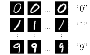
6.1. Input Data
As the input data, we use the well-known MNIST database of handwritten digits. As the input data, we have 28×28 pixel grey-scale images. Each image has a natural label which is the digit that the image represents:
In order to estimate the efficiency of the model that we’re going to build, we split the input data into training and test sets:
DataSetIterator train = new RecordReaderDataSetIterator(...);
DataSetIterator test = new RecordReaderDataSetIterator(...);
Once we have the input images labeled and split into the two sets, the “data elaboration” stage is over and we may pass to the “model building”.
6.2. Model Building
As we’ve mentioned, there are no models that work well in every situation. Nevertheless, after many years of research in ML, scientists have found models that perform very well in recognizing handwritten digits. Here, we use the so-called LeNet-5 model.
LeNet-5 is a neural network that consists of a series of layers that transform the 28×28 pixel image into a ten-dimensional vector:
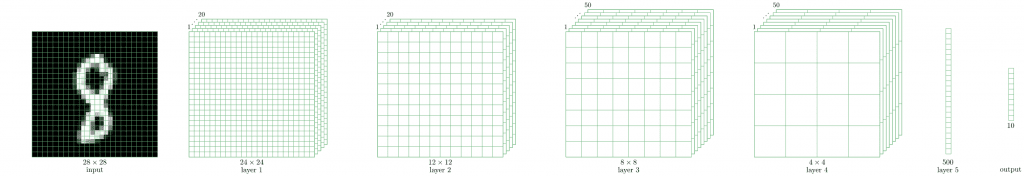
The ten-dimensional output vector contains probabilities that the input image’s label is either 0, or 1, or 2, and so on.
For example, if the output vector has the following form:
{0.1, 0.0, 0.3, 0.2, 0.1, 0.1, 0.0, 0.1, 0.1, 0.0}it means that the probability of the input image to be zero is 0.1, to one is 0, to be two is 0.3, etc. We see that the maximal probability (0.3) corresponds to label 3.
Let’s dive into details of model building. We omit Java-specific details and concentrate on ML concepts.
We set up the model by creating a MultiLayerNetwork object:
MultiLayerNetwork model = new MultiLayerNetwork(config);In its constructor, we should pass a MultiLayerConfiguration object. This is the very object that describes the geometry of the neural network. In order to define the network geometry, we should define every layer.
Let’s show how we do this with the first and the second one:
ConvolutionLayer layer1 = new ConvolutionLayer
    .Builder(5, 5).nIn(channels)
    .stride(1, 1)
    .nOut(20)
    .activation(Activation.IDENTITY)
    .build();
SubsamplingLayer layer2 = new SubsamplingLayer
    .Builder(SubsamplingLayer.PoolingType.MAX)
    .kernelSize(2, 2)
    .stride(2, 2)
    .build();
We see that layers’ definitions contain a considerable amount of ad-hoc parameters which impact significantly on the whole network performance. This is exactly where our ability to find a good model in the landscape of all ones becomes crucial.
Now, we are ready to construct the MultiLayerConfiguration object:
MultiLayerConfiguration config = new NeuralNetConfiguration.Builder()
    // preparation steps
    .list()
    .layer(0, layer1)
    .layer(1, layer2)
    // other layers and final steps
    .build();
that we pass to the MultiLayerNetwork constructor.
6.3. Training
The model that we constructed contains 431080 parameters or weights. We’re not going to give here the exact calculation of this number, but we should be aware that just the first layer has more than 24x24x20 = 11520 weights.
The training stage is as simple as:
model.fit(train);
Initially, the 431080 parameters have some random values, but after the training, they acquire some values that determine the model performance. We may evaluate the model’s predictiveness:
Evaluation eval = model.evaluate(test);
logger.info(eval.stats());
The LeNet-5 model achieves quite a high accuracy of almost 99% even in just a single training iteration (epoch). If we want to achieve higher accuracy, we should make more iterations using a plain for-loop:
for (int i = 0; i < epochs; i++) {
    model.fit(train);
    train.reset();
    test.reset();
}
6.4. Prediction
Now, as we trained the model and we are happy with its predictions on the test data, we can try the model on some absolutely new input. To this end, let’s create a new class MnistPrediction in which we’ll load an image from a file that we select from the filesystem:
INDArray image = new NativeImageLoader(height, width, channels).asMatrix(file);
new ImagePreProcessingScaler(0, 1).transform(image);
The variable image contains our picture being reduced to 28×28 grayscale one. We can feed it to our model:
INDArray output = model.output(image);The variable output will contain the probabilities of the image to be zero, one, two, etc.
Let’s now play a little bit and write a digit 2, digitalize this image and feed it the model. We may get something like this:
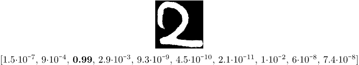
As we see, the component with maximal value 0.99 has index two. It means that the model has correctly recognized our handwritten digit.
7. Conclusion
In this tutorial, we described the general concepts of machine learning. We illustrated these concepts on logistic regression example which we applied to a handwritten digit recognition.