

Yes, we're now running our only Summer Sale. All Courses are 30% off until 20th July, 2026:
Learn through the super-clean Baeldung Pro experience:
>> Membership and Baeldung Pro.
No ads, dark-mode and 6 months free of IntelliJ Idea Ultimate to start with.
1. Overview
In this tutorial, we’ll dissect transformers to gain some intuition about how they represent text. Next, we’ll learn about a very cool model derived from it named BERT and how we can use it to obtain richer vector representations for our text.
To understand the following content, some basic knowledge about general Deep Learning and Recurrent Neural Networks is required.
Let’s begin!
2. What Are Transformers?
Transformers are big encoder-decoder models able to process a whole sequence with a sophisticated attention mechanism.
The most advanced architectures in use before Transformers were Recurrent Neural Networks with LSTM/GRU.
These architectures, however, have the following problems:
- They struggle with really long sequences (despite using LSTM and GRU units)
- They are fairly slow, as their sequential nature doesn’t allow any kind of parallel computing
Transformers work differently:
- They work on the whole sequence, which let them learn long-range dependencies
- Some parts of the architecture can be processed in parallel, making training much faster
They were presented in the popular paper Attention Is All You Need, named like that because of the new attention model proposed in it.
3. Dissecting the Transformer
3.1. Overall Architecture
Let’s imagine we want to translate “My tailor is rich” from English to Spanish. Then, the transformer would look like this:
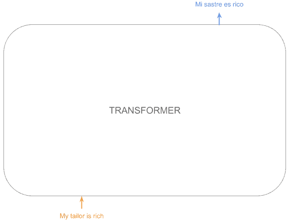
As mentioned before, it is a big encoder-decoder model where the input sequence gets into a big encoding block, obtaining rich embeddings for each token, which will feed the decoding block to obtain an output.
So the previous diagram would look like this:
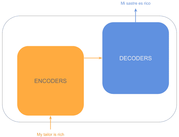
Now, each of the encoding/decoding blocks actually contains many stacked encoders/decoders. That way, the initial layers capture more basic patterns, whereas the last layers can detect more sophisticated ones, similar to convolutional networks:
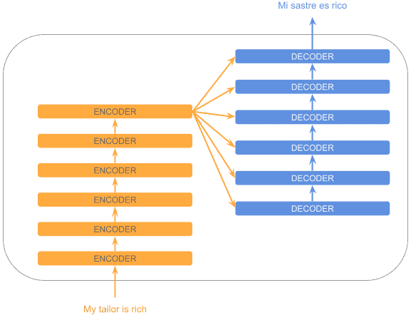
As we can see, the last encoder output is used by every decoder.
3.2. Input
Encoders can’t operate directly with text but with vectors. So how do we obtain those vectors?
The text must be converted into tokens, which are part of a fixed vocabulary.
After that, tokens are converted into embedding vectors by using a fixed representation like word2vec or any other.
But, because we are processing the sequence all at once, how can we know the position of tokens in the sequence? To address this problem, the transformer adds a positional encoding vector to each token embedding, obtaining a special embedding with positional information.
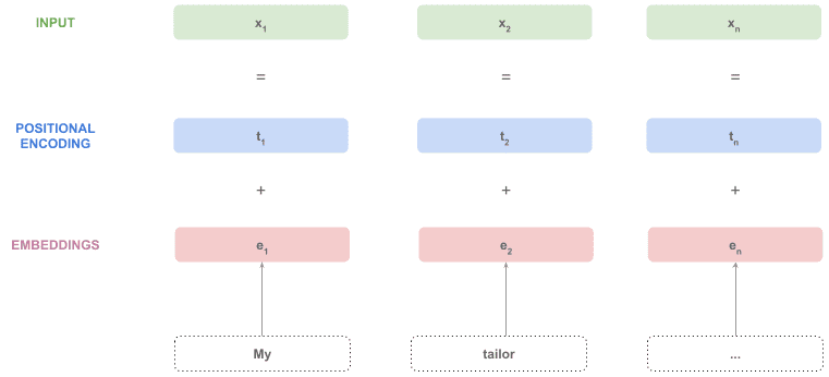
Those vectors are ready to consume by the encoders.
3.3. The Encoder Stack
The encoder receives one vector per token in the sequence  , and returns a new vector per token with the same shape as the input sequence
  .
.
Intuitively, the encoder is returning the same input vectors but “enriched” with more complex information.
So, for now, we have a black box receiving one vector per token and returning one vector per token:
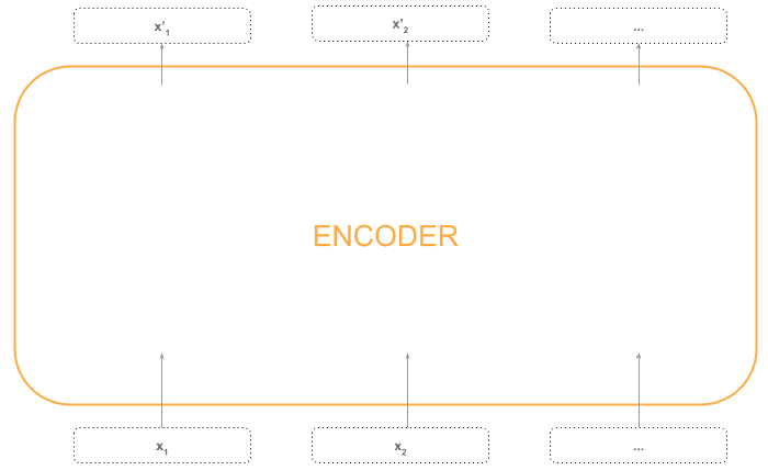
Let’s open the box and see what’s in it.
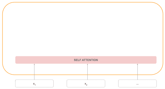
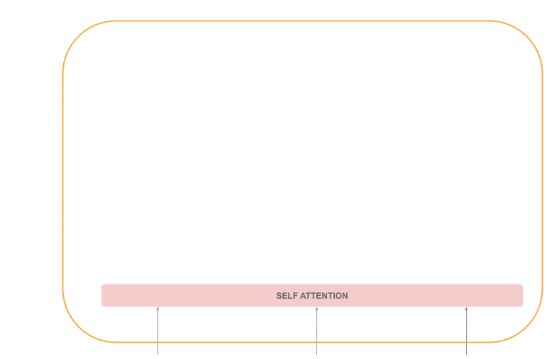
The very first layer in the encoder is the self-attention layer, which is the most important part of the encoder. This layer can detect related tokens in the same sequence, no matter how far they are.
For example, in the sentence: “The cat is on the mat. It ate a lot of food”, “It” refers to the cat, and not the mat, so the attention mechanism will weigh the token “cat” in the processing of token “It”.
This part of the process is sequential, as the attention layer needs the whole sequence:
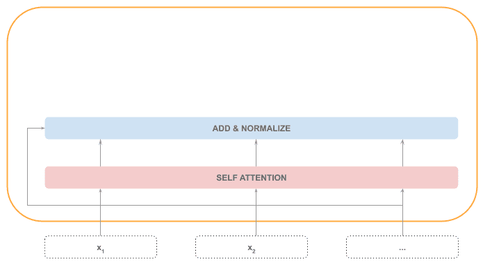
Next, we find an “Add & Normalize” layer, which adds the self-attention output with the input sequence and then normalizes it. This part of the processing is also sequential, given the normalization step requires the whole sequence.
After that, each token is processed by a feed-forward neural network, a step that can be processed in parallel:
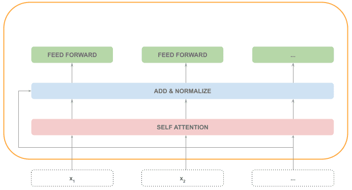
Finally, another Add & Normalize step is applied with the input and output of the feed-forward step:
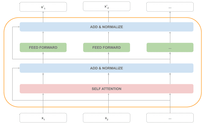
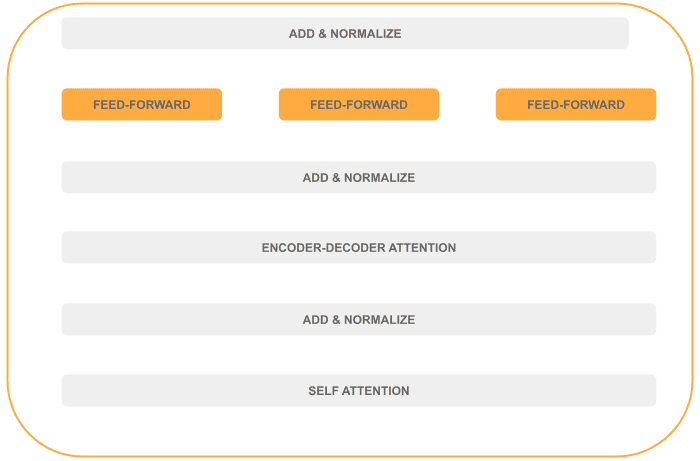
In the picture below, we can see the distribution of sequential (in gray) and parallel (in orange) steps inside the encoder:
The current encoder input will be processed producing the input of the following one: , except in the case of the last encoder, whose output will be considered the output of the whole encoding stack.
The animation below illustrates the process:

3.4. The Decoder Stack
The decoder is pretty much an encoder but with an additional encoder-decoder attention layer.
The inputs of every decoder are:
- Previously generated sequence
- Encoder’s output
Seeing it as a black box, this would look like this:
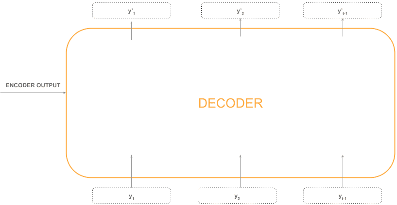
Let’s analyze what’s inside a decoder.
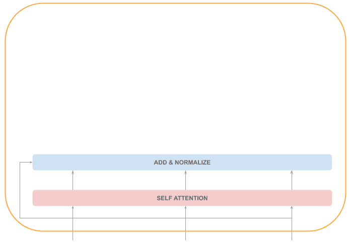
The first layer is again a self-attention layer, so the execution is sequential. The decoder self-attention layer is different from the encoder’s because we don’t have the whole sequence.
The output sequence is created token by token, so when we are processing the token at position “t”, we only have the sequence from the beginning up to the previous position: 
After that, we’ll have the already familiar “Add & Normalize” layer:
The next step is the one that makes the difference with the decoder: the encoder-decoder attention layer.
This attention mechanism provides insight into which tokens of the input sequence are more relevant to the current output token.
This step is sequential and is followed by an “Add & Normalize” layer:
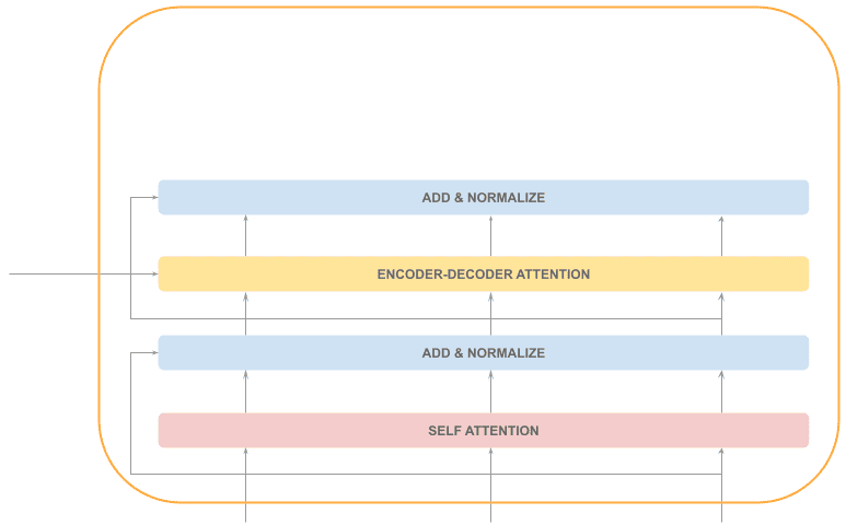
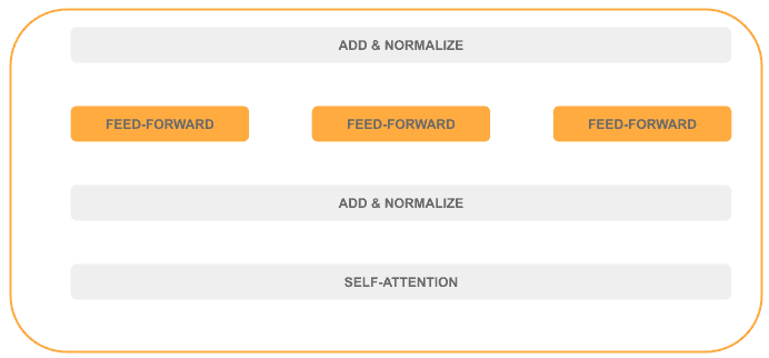
Finally, we also have a feed-forward layer (parallelizable), followed by an “Add & Normalize” layer:
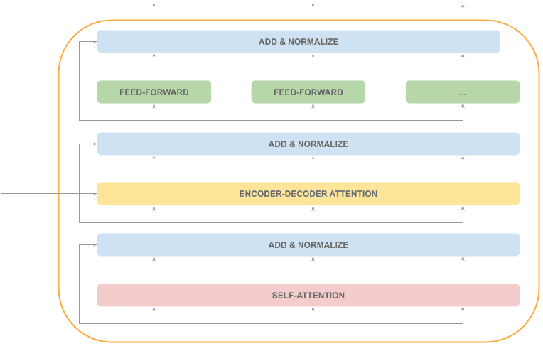
As we can see, most of the decoder processing is sequential (in gray), and just one layer can be processed in parallel (in orange):
The current decoder input  will be processed producing an output:
  , which will feed the next decoder.
The last decoder is connected to the output layers (we’ll get into that soon), generating the next output token. The process continues until the generated token is a special one meaning “end of the sentence”.
This animation summarizes the decoder process:
3.5. Output
We learned that decoders produce a list of output vectors for the tokens previous to the position being processed. Therefore, will be processed producing a similar sequence: but richer, semantically speaking.
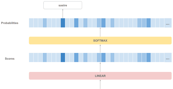
If those tokens represent the already generated sequence, how do we generate the next token?
The decoder stack outputs a vector of floats. This vector is connected to a linear layer, a fully connected neural network projecting the output vector into a large vector with the same size as the vocabulary. That vector is named the “logits” vector and contains a score for each token in the vocabulary.
Finally, that layer is connected to a softmax layer so that scores are converted into probabilities. That way, we have a vector containing the probability of every token to be the next in the sequence. All we have to do is taking the token with the highest probability in the probabilities vector.
Let’s see it in a diagram:
4. BERT
4.1. Description
BERT is just a pre-trained Transformer encoder stack.
It was one of the biggest achievements in NLP, as it allows, with little training effort, to fine-tune the model for our specific task.
It is the equivalent to image processing pre-trained models, which allow us to classify new objects without much training, as the biggest training effort to learn more basic features is already provided.
Similarly, we could add a couple of dense layers on top of BERT’s output and create a classifier in a different language domain. It would take some time to adapt to the differences in vocabulary, syntax, language model, and so on, but the basic learning is already contained in the model.
4.2. How BERT Operates
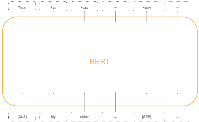
To use BERT, we need a vocabulary with two special tokens: [CLS] and [SEP].
The first input token must be a special [CLS] token that stands for “Classification”, and the sequence must finish with the token [SEP], which stands for “Separator”.
Bear in mind BERT always receives a fixed sequence of vectors (a typical size would be 512), so we need to indicate where the sequence ends if it’s shorter.
See an example in the diagram below:
4.3. Text Embeddings
If we want a vector representing each token, we can just use the corresponding output vector produced by the encoding stack block (The “y” vectors in the diagram above)
If we need a vector representing the whole sequence, there are 3 strategies we can follow:
- Use the [CLS] token output vector
- Apply mean pooling between the token vectors
- Apply max-pooling between the token vectors
The default strategy is the first one, though some papers suggest the other two work best for other tasks.
5. Conclusion
In this tutorial, we learned what transformers are, their building blocks, and why they work so well, thanks to their advanced attention model.
Finally, we briefly knew what BERT is and how we can obtain text embedding vectors by using it.