

Yes, we're now running our only Summer Sale. All Courses are 30% off until 20th July, 2026:
A Simple Explanation of Naive Bayes Classification
Last updated: August 30, 2024
Learn through the super-clean Baeldung Pro experience:
>> Membership and Baeldung Pro.
No ads, dark-mode and 6 months free of IntelliJ Idea Ultimate to start with.
1. Overview
In this article, we’ll study a simple explanation of Naive Bayesian Classification for machine learning tasks.
By reading this article we’ll learn why it’s important to understand our own a prioris when performing any scientific predictions. We’ll also see how can we implement a simple Bernoulli classifier which uses Bayes’ Theorem as its predicting function.
By the end of this article, we’ll have an intuitive understanding of one of the most fundamental theorems in statistics, and we’ll have seen one of its possible algorithmic implementations.
2. Bayes’ Theorem
Let’s start with the basics. This is Bayes’ theorem, it’s straightforward to memorize and it acts as the foundation for all Bayesian classifiers:

In here,  and
and  are two events,
  and
and  are the two probabilities of A and B if treated as independent events, and
  and
and  is the compound probability of A given B and B given A, respectively.
and are the crucial points here, and they refer to the so-called a priori probabilities of A and B.
3. What Are A Priori Probabilities and Why Do They Matter?
3.1. The Meaning of A Priori
A priori is a Latin expression which means unverified or not tested, but also assumed or presumed.
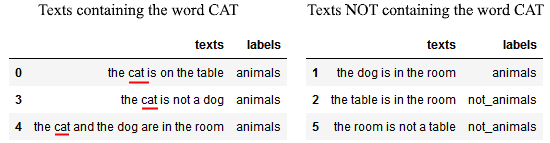
So what does it mean for the probability of an event to be unverified or presumed? Let’s use the following thought experiment as an example, to which we’ll refer for the rest of this article. We’re playing a guessing game, based upon the following corpus of texts:
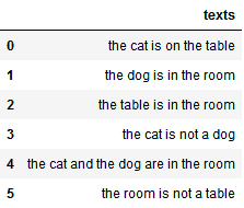
3.2. The Game We Are Playing
In this game, we must guess whether a text in a language we don’t speak, English, talks about a concept we don’t understand, animals. Each text in the corpus above talks, or not, about animals, and we can read all texts as many times as we want before we start guessing.
When we start the game, the game host will show us a new text, previously unseen, and ask us to correctly guess whether it talks about animals or not:

Of course, any English speaker can immediately identify which texts belong to which category, but let’s imagine that we don’t speak the language and can’t thus rely on semantic clues for solving the task. In that case, we could still make simple guesses on the basis of the frequencies of occurrence of classes and/or features over the total of observations.
This type of game is called, in Natural Language Processing, text classification. The way we’ll approach it is by making simple guesses first, and later building them up in complexity as we acquire more insight into the structure of the data.
4. How to Make Bayesian Guesses
4.1. Can We Guess With No Prior Knowledge?
We don’t yet know how the classes are distributed among the texts we’ve read, or in general, in the linguistic system we’re studying. Remember, we don’t speak English. This situation corresponds to the lack of any a priori knowledge on the behavior of the system, in relation to the predictions we must perform.
Under this circumstance, without any prior knowledge, we can’t perform any predictions at all.
This is strongly counter-intuitive: we might in fact argue that a good guess would be to classify half of the texts as animals, and half of them as not_animals. We’d then randomly draw from a uniform distribution, and assign a label according to the result of our draw, and whether this is higher or lower than the median value for that distribution.
4.2. No Predictions Without Prior Knowledge
Unfortunately, we can’t do that so freely: otherwise, we’d be adding an additional hypothesis on the behavior of the system, which corresponds to the addition of a priori knowledge, and which in turn negates the underlying hypothesis for this paragraph.
This makes the assignment of prior probabilities to the class affiliation of texts a required extra hypothesis to perform any guesses.
Prediction without a priori knowledge is therefore not possible.
But because the game host understands that our task is impossible as it stands now, they kindly provide us with some extra information. Specifically, they provide us with a list of class labels associated with the texts we’ve read:
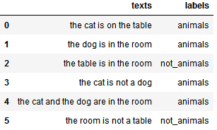
4.3. Guessing With Prior Knowledge on the Class Distribution
We can now formulate a base prediction on the class affiliation of an unseen text, on the basis of the additional information that we just received:
Guess 1: Any new text belongs to the class which most frequently appears in the observed corpus.
This guess is straightforward to understand. Given that four out of six observed texts talk about animals, we then deduce that an unobserved text is also likely to talk about animals.
To perform this guess we need no knowledge on the features of the corpus or their relation with the class affiliation of a text, nor any understanding of the language for that matter. In fact, we could delete the content of the texts from the table above, and still be able to perform this prediction:

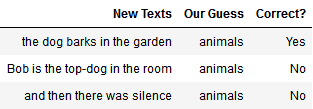
The simple prediction rule says: if you see a new text, classify it as animals because this class is the most frequent. Because there are two classes, and because the class of animals is the most likely one, we’re always going to guess that a new text belongs to it:
The predictions are unsatisfactory, but we haven’t yet made use of the features of the text, which we can discuss now.
4.4. Guessing With Prior Knowledge on Class and Feature Distribution
We can then imagine that not all words equally relate to the same concept and that some words in a text are more frequently associated with the target class, animals, than others.
It’s important to note that this assumption is largely arbitrary: the text “this isn’t a text about animals” doesn’t talk about animals, by definition, and yet contains the word corresponding to the class label itself. This assumption, however, allows us to guess the classes of unseen texts, as follows:
Guess 2: If a word contained in a new text was previously seen in a text belonging to the target class, the new text is more likely to belong to the target class.
By making this assumption we could then proceed to read all texts in the corpus and score each word according to their likelihood to be present in a text that talks about animals.
This is done as follows. First, we start with the first word of the first text, the article THE. We then divide the corpus into two sets, grouped according to the presence of the word:
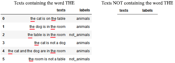
We can then ask ourselves how likely is it that, if a text talks about animals, it also contains the word THE. This is done by replacing the events A and B indicated in Bayes’ theorem, above, with the events “text labeled as animals” and “text contains the word THE”, respectively:

We can see something important here. Knowing that the word THE is present in a text doesn’t teach us anything we didn’t know about that text. More specifically, it doesn’t give us any better guesses than we could already make with the previous guessing rule.
4.5. A More Informative Word
We then proceed with the second word of the first sentence, and repeat the same procedure:
The word CAT is more informative than the word THE, as we could expect if we knew English. It appears that the majority of the texts labeled as animals, and specifically 75% of them, contain it. At the same time, none of the texts labeled as not_animals contain it.
This means that the word CAT is both sensitive and specific in predicting the class affiliation of a text:

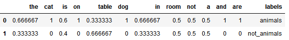
That seems like a very good result and is significantly more informative than the previous one. We can then repeat the same process for all words for all texts. If we do so, we can build a distribution of conditional probabilities of class affiliation given the text features:
5. The Danger of Having High Confidence on Our A Priori Knowledge
We could stop now, and use the table obtained above as a lookup table containing rules for our guesses. Notice how some of the words have a probability of being affiliated with the class animals which equals one.
We could therefore simply label a text as belonging to that class whenever we read one of those words:
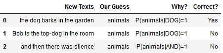
This type of approach, however, of having absolute confidence in our a priori knowledge on the behavior of a system, is extremely dangerous when performing predictions. It leads in fact to disregarding all evidence contrary to assumptions on which we have absolute, or 100%, confidence.
6. An Intuitive and Rationalist Interpretation of Bayes’ Theorem
6.1. Without Assumptions, There Can Be No Predictions
The small thought experiment we’ve discussed shows us something important. It’s very hard, and in fact impossible, to perform predictions without a large amount of background knowledge on the system that we study.
This leads to an important consideration, which is the foundation for the rationalist interpretation of Bayes’ theorem. We can’t perform any predictions at all unless we have prior assumptions on the general behavior of a system.
If we have those assumptions, those a prioris with Bayesian terminology, we can then perform predictions. Our predictions then become as valid as the validity of the underlying assumptions.
6.2. Assumptions Are Good but Use Them in Moderation
A subtle problem, common to both human and machine classifiers, is the one that relates to high confidence in a prioris. By increasing the number of assumptions or our reliability on them, we generally increase the accuracy of our predictions. After a certain point, however, this is problematic.
More prior assumptions or higher confidence in them generally prevent the acquisition of new knowledge. In machine learning terms, it leads to the overfitting of the model on the training dataset and to poor capacity for generalization.
6.3. The Middle Way Is the Best Way
We can then draw the following conclusion. We learned that both absolute trust in our knowledge and absolute ignorance should be avoided. The way forward is to then have a certain amount of confidence in our own knowledge but to remain willing to update it as new evidence emerges in favor or against it.
This rationalist interpretation of Bayes’ Theorem applies well to Naive Bayesian Classifiers. What the classifier does during training is to formulate predictions and make hypotheses. These are then tested against observations (the training dataset), and discrepancies between observations and predictions are noted.
The classifier then increases or decreases its confidence in those hypotheses according to whether the evidence supports or refuses them.
7. A Bernoulli Naive Bayesian Classifier
If we’re interested in trying out this corpus in a simulation of their own, the following code uses Python 3+, Pandas and skLearn, to implement Bayes’ Theorem to learn the labels associated with the sample corpus of texts for this article:
import pandas as pd
from sklearn.feature_extraction.text import CountVectorizer
from sklearn.naive_bayes import BernoulliNB
corpus = ['the cat is on the table','the dog is in the room','the table is in the room','the cat is not a dog',
    'the cat and the dog are in the room','the room is not a table']
labels = ['animals','animals','not_animals','animals','animals','not_animals']
df = pd.DataFrame({'Texts':corpus,'Labels':labels})
cv = CountVectorizer(token_pattern='\w+')
BoW = cv.fit_transform(df['Texts'])
classifier = BernoulliNB()
classifier.fit(BoW,df['Labels'])
predictions = classifier.predict(BoW)
df['Predictions']=predictions
print(df)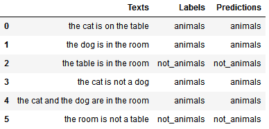
8. Conclusions
Bayes’ Theorem states that all probability is a conditional probability on some a prioris. This means that predictions can’t be made unless there are unverified assumptions upon which they are based.
At the same time, it also means that absolute confidence in our prior knowledge prevents us from learning anything new.
The way forward is therefore the middle. With the middle way, we update our knowledge on the basis of new evidence that arises in support or contradiction of it.