

Learn through the super-clean Baeldung Pro experience:
>> Membership and Baeldung Pro.
No ads, dark-mode and 6 months free of IntelliJ Idea Ultimate to start with.
Learn through the super-clean Baeldung Pro experience:
>> Membership and Baeldung Pro.
No ads, dark-mode and 6 months free of IntelliJ Idea Ultimate to start with.
In this tutorial, we’ll study how to normalize the features of a table or dataset.
We’ll start by discussing why normalization is useful and when we are expected to apply it. Then, we’ll see the three most common methods for normalizing features in a table.
At the end of this tutorial, we’ll be familiar with the notion of normalization and the formulas for its most common implementation.
The idea of normalization exists because, in general, we should expect a new dataset to not be normalized. It is, however, often desirable to normalize a dataset on which we plan to train a machine learning model. We’ll see shortly what this means, but for now, it’s important to get an intuitive understanding as to why this is the case.
Let’s consider the distribution of weight and height in a class of students comprising 5 persons:
| Student | Weight (Kg) | Height (cm) |
|---|---|---|
| Dotty | 89 | 182.1 |
| Hamza | 68 | 146.8 |
| Devonte | 75 | 170.5 |
| Alex | 68 | 154.8 |
| Reiss | 86 | 180.6 |
This is the corresponding scatterplot:
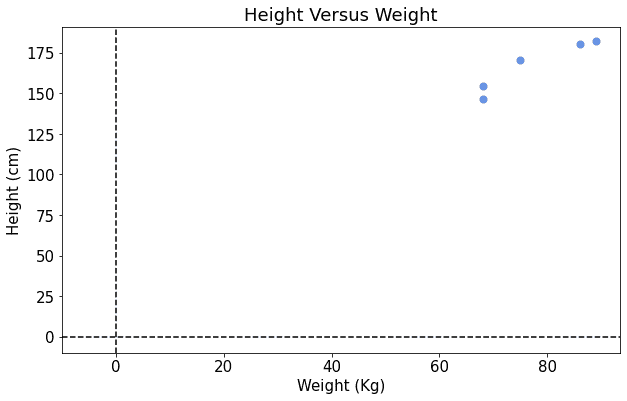
By looking at the figure above, we can get the idea that some kind of relationship exists between the two features, weight, and height. More accurately, we can suspect the relationship to be linear, and we may want to identify a model that fits it.
A linear model  comprises two parameters, the slope
  and the intercept
  . Because we do not know exactly what linear model will fit this dataset, we can start by assigning random values to and . Let’s say, for simplicity, that we initially assign 0 to both and :
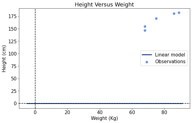
If we do that, we can see that our model is inaccurate for two reasons: it’s too low in the plot, and it’s also too flat. We can then increase both the values of and by a little and see whether the line gets closer to the observations:
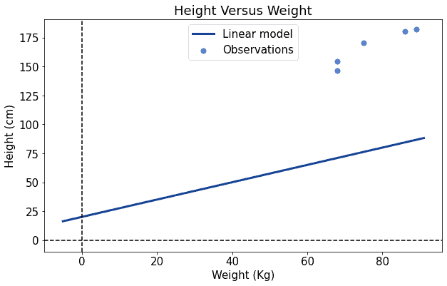
It looks better now. We can then repeat the process of increasing the parameters, the values of and . We do this until we’re satisfied with our fit:
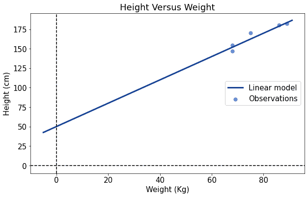
This approach can work, although it may take quite a few iterations before convergence.
However, it would have been better for us if our dataset were somewhat centered around the origin. If that had been the case, then we wouldn’t have needed to search so widely for the correct parameters in our model. Let’s look at thi2.1. What is Normalization, Intuitively?s second table and at its corresponding scatterplot:
| Student | Weight | Height |
|---|---|---|
| Dotty | 0.562 | 0.429 |
| Hamza | -0.438 | -0.571 |
| Devonte | -0.105 | 0.100 |
| Alex | -0.438 | -0.344 |
| Reiss | 0.419 | 0.386 |
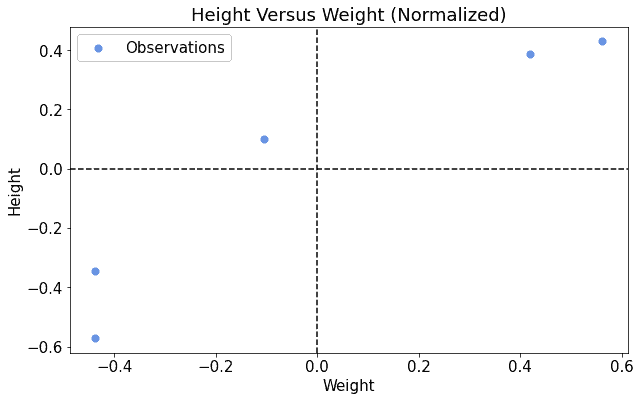
As in the previous case, we want to find a linear model that fits the data. In this second case, it seems that a line that passes through the origin, or very close to it, may do the job. As in the previous case, we initialize the parameters and of the linear model to 0:
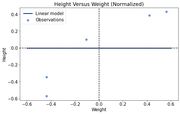
This time, though, it seems that the intercept is already in the correct position, or at least very close to it. This means that we need to increase the slope of the line, but we don’t need to touch the intercept by much:
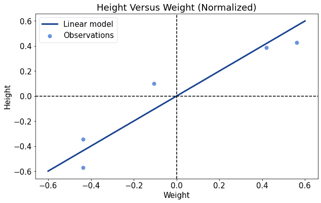
This time the training process was significantly faster, and it required less movement in the parameter space before reaching convergence.
Now, the two tables we used in these examples are related to one another. In fact, we call the second table the normalized version of the previous table. The process through which these two datasets are related is subsequently called normalization.
The examples we studied above indicate two typical cases in machine learning. The first one corresponds to a table comprising raw measurements from the environment, which didn’t receive any preprocessing. This situation generally requires a longer training process for a machine learning model.
The second case corresponds to a preprocessed dataset, where the features have already been manipulated to fit into some specific range or interval or to have some specific shape. This generally leads to faster training times for our models.
If we don’t have any specific reason for avoiding it, it’s a good habit to normalize a dataset before training a machine learning model on it. This should, in the best case, significantly improve the training time. In the worst case, we have simply added a few subtractions and divisions to the list of operations in our machine learning pipeline.
We should now discuss some mistakes that are common when studying the concept of normalization for the first time. The first is the risk of confusing the normalization of a distribution with a normal distribution. A normal distribution isn’t necessarily the result of normalization, though it could be, and as a consequence, the two concepts must be kept separated.
We can think of normalization as a process or procedure through which we assign new values to the features in distribution, according to a specified set of rules. We can instead think of normal distributions as distributions with a particular shape, the typical Gaussian bell.
We also need to keep in mind that the word normalization isn’t unambiguous either. In some cases, the term describes the process of mapping a probability distribution to another. In others, it describes the scaling of a variable to a particular interval.
It’s therefore important when we’re studying an article on statistics or machine learning to make sure that we understand exactly what an author means with the word normalization.
Another frequently encountered word that sometimes overlaps with normalization is standardization. The latter, however, refers to the process of mapping a distribution to a Gaussian distribution centered around the origin, specifically, and should not be confused with the former.
We can now approach the actual methods for normalizing a feature in a table. We’ll see three here that compose our basic arsenal of normalization techniques for a new raw dataset.
The first corresponds to the mapping of the distribution to the unit interval. Because the unit interval is ![[0, 1]](/wp-content/ql-cache/quicklatex.com-944fdd98d4f1854c8720f98d8b20b6ad_l3.svg "Rendered by QuickLaTeX.com") , we want the lowest value in the distribution to map to zero and the greatest value to map to 1 or to get as close to 1 as possible.
, we want the lowest value in the distribution to map to zero and the greatest value to map to 1 or to get as close to 1 as possible.
Let’s decompose these requirements, and call  the map we use on the variable
  . If
. If  , this means that the analytical formula of must include the expression
  . If the codomain of corresponds to , then its range is 1; thus if has a range of
  , the analytical formula of must include a division by
  .
.
The complete formula for normalization to the unit interval is, therefore:

Here is a chart that shows how we can normalize to the unit interval the distribution of weights and heights that we used as an example above:
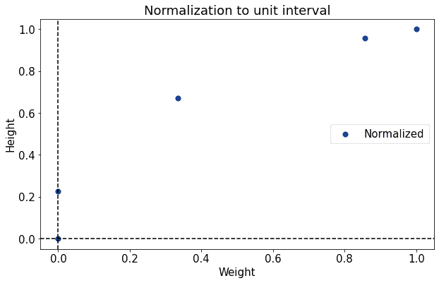
When applying this type of normalization, we must be careful to ensure, as we divide for the range of the original distribution, that this range is greater than zero.
Sometimes we might, however, be interested in highlighting information about the relationship between each observation and the mean of its distribution. To do that, we can first shift the distribution to the left by subtracting for the mean  :
:

By doing this, all values lower than become negative, while all values higher than that become positive. This type of normalization is also frequently accompanied by scaling. Scaling corresponds to the division by the range of the original distribution, similarly to what we saw in the previous case:

This is the particular method for normalization that we employed for the table shown in the section above.
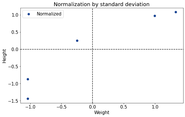
Finally, we can also normalize a distribution by leveraging its standard deviation. This is particularly useful if our original distribution is normal, as the resulting distribution will have a mean of 0 and a standard deviation  of 1:
of 1:

This is the example bivariate distribution we used, normalized by means and standard deviations:
The determination of the type of normalization to use depends, as it’s common in machine learning, on the task we’re performing. It’s appropriate when we’re working on a new dataset to test some alternative normalization techniques and see which one leads to improvements in the accuracy of our models.
The selection of a specific normalization technique for a given task is therefore done heuristically, and we should try a few techniques to find out which one works best.
In this article, we studied how to normalize the features of a table or dataset.
We first learned what normalization is and how it functions from an intuitive perspective. Then, we studied the common mistakes one can make when approaching the subject for the first time.
Finally, we studied the main techniques for normalization and their associated formulas.