

Learn through the super-clean Baeldung Pro experience:
>> Membership and Baeldung Pro.
No ads, dark-mode and 6 months free of IntelliJ Idea Ultimate to start with.
Learn through the super-clean Baeldung Pro experience:
>> Membership and Baeldung Pro.
No ads, dark-mode and 6 months free of IntelliJ Idea Ultimate to start with.
In this tutorial, we’ll explain how to perform cross-validation of decision trees. We’ll also talk about interpreting the results of cross-validation.
Although we’ll focus on decision trees, the guidelines we’ll present apply to all machine-learning models, such as Support Vector Machines or Neural Networks, to name just two.
A decision tree is a plan of checks we perform on an object’s attributes to classify it. For instance, let’s take a look at the decision tree for classifying days as suitable for playing outside:
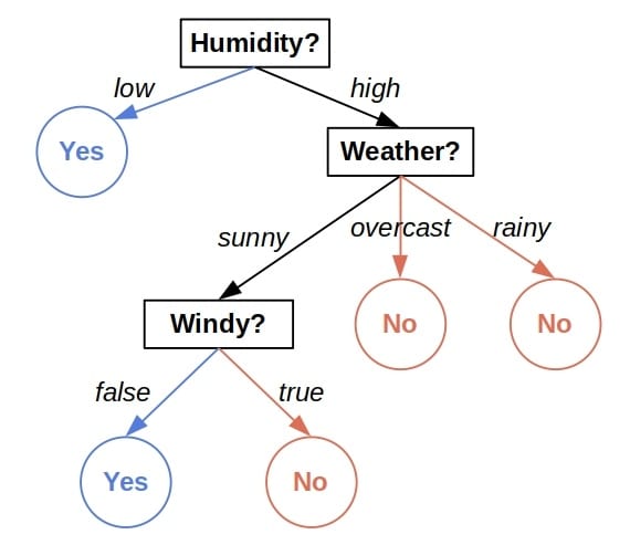
Given the attributes of a day, we start at the top of the tree, inspect the feature indicated by the root and visit one of its children depending on the feature’s value. Then, we repeat the process until we reach a leaf node and read the decision.
Two kinds of parameters characterize a decision tree: those we learn by fitting the tree and those we set before the training. The latter ones are, for example, the tree’s maximal depth, the function which measures the quality of a split, and many others.
They also go by the name of hyper-parameters, and their choice can significantly affect the performance of the decision tree. So, a natural question is how to set the hyper-parameters to increase the performance of the resulting tree as much as possible. To do that, we usually conduct cross-validation.
First, we need to decide which hyper-parameters we’ll tune. The thing is that there are a lot of them, and rigorously testing each combination of values can take too much time. For instance, let’s say that we decided to work with two hyper-parameters:
 : the maximal depth of the tree.
 : the function to measure the quality of a split.
Next, we identify which hyper-parameter values we want to test. For example,  , and
, and  , where
  is the information gain, and
  is the Gini impurity. That way, we get a grid of
  combinations:
![\[\begin{matrix} d & q \\ 4 & Gini \\ 4 & Gain \\ 5 & Gini \\ 5 & Gain \\ \end{matrix}\]](/wp-content/ql-cache/quicklatex.com-e8df9a85138df8a88e4ce9aa563f70ba_l3.svg "Rendered by QuickLaTeX.com")
We’ll train and validate a tree using every combination from the grid.
The usual way to cross-validate a tree is as follows. We split the data into the training and test sets. Then, we split the training data into  folds:
  (
( , or more, depending on our computational capacities). When dealing with classification problems, the best practice is to keep the ratio of different classes in each fold approximately the same as in the entire dataset.
Afterward, we iterate over the folds. In the  -th pass, we use all the folds but
  to train a tree for each combination in the grid, validating the fitted tree on the reserved fold . That way, we get
  trees and validation scores for each grid combination.
If there are  combinations in the grid, and we split the training set into folds, we’ll have an
  table of validation scores. Each score results from testing the tree on the fold we didn’t use to train it. Visually, it’s a two-dimensional matrix:
![\[\begin{matrix} score_{1, 1} & score_{1, 2} & \ldots & score_{1, m} \\ score_{2, 1} & score_{2, 2} & \ldots & score_{2, m} \\ \ldots \\ score_{r, 1} & score_{r, 2} & \ldots & score_{r, m} \end{matrix}\]](/wp-content/ql-cache/quicklatex.com-b3350381b1ada5d3cf3e4ca9e6ade22c_l3.svg "Rendered by QuickLaTeX.com")
The value  is the performance score we get by training the tree on folds other than
  using the
  combination in the hyper-parameter grid and evaluating it on . For example, if we measure accuracy, we may get the results like this with
  :
:
![\[\begin{matrix} d & q & & & & & \\ 4 & Gini & 0.85 & 0.87 & 0.87 & 0.91 & 0.85\\ 4 & Gain & 0.81 & 0.82 & 0.87 & 0.85 & 0.80\\ 5 & Gini & 0.93 & 0.93 & 0.89 & 0.91 & 0.95\\ 5 & Gain & 0.90 & 0.91 & 0.93 & 0.89 & 0.91 \end{matrix}\]](/wp-content/ql-cache/quicklatex.com-0472c74c0b49723b6aab825c75396638_l3.svg "Rendered by QuickLaTeX.com")
Finally, we set the hyper-parameters to the combination which gave the best tree. Usually, we go with the settings having the best mean value. However, means can mislead us if we don’t account for the variability of scores. For instance, the mean accuracy for  in the above table is
  , while the mean accuracy for
  is
is  :
:
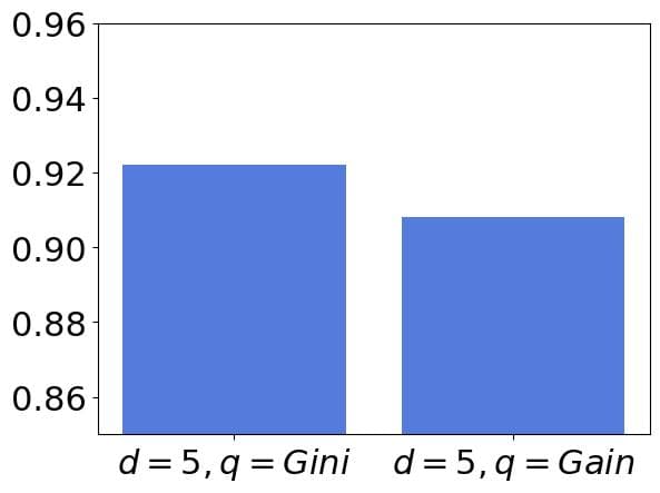
As the accuracy difference of  can be substantial in the domain where we will use the tree, we could conclude that the combination allows for training more accurate trees. But, if we calculate the standard deviations and add the margin errors, we’ll see that the intervals overlap:
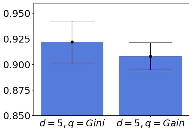
In such cases, we should choose the computationally less intensive settings or those that lead to simpler models. For instance, if we considered only the depth hyper-parameter and the intervals for  and
and  overlapped, we’d go with
  . The reason is that the shallower trees work faster and are easier to understand
Alternatively, we could calculate additional performance scores to break ties or look for the combination(s) in the Pareto front of scores. Another option is to run a statistical test on the scores to find which combination provides the most accurate trees.
However, we should keep in mind that even if we found a statistical difference between two combinations’ scores, that wouldn’t mean that the trees trained under one hyper-parameter setting are necessarily better than those trained under the other combination. For instance, we may consider the trees whose mean accuracy scores are within  the same even if the error bars overlap.
That’s how cross-validation is usually done in practice. However, the approach has a shortcoming. Since we first split the data into the training and test sets and then cross-validate the tree using the folds of the training set, our results are conditional on the main train/test split. If our dataset is small, the final tree’s performance on the test set can be an imprecise estimate of its actual performance.
Nested cross-validation addresses this issue by iterating over data splits as well. Namely, we split the data into the training and test folds  times. Further, we perform the cross-validation as described above for each of the
  splits.
That way, we eliminate the effect of data splits (if any) and avoid sampling bias. But, the main disadvantage is that we do times more work, which we may not be able to afford.
Here’s an example of the result matrix of the nested cross-validation with  outer and inner splits:
![\[\begin{matrix} split & d & q & & & & & \\ \hline \\ 1 & 4 & Gini & 0.85 & 0.87 & 0.87 & 0.91 & 0.85\\ 1 & 4 & Gain & 0.81 & 0.82 & 0.87 & 0.85 & 0.80\\ 1 & 5 & Gini & 0.93 & 0.93 & 0.89 & 0.91 & 0.95\\ 1 & 5 & Gain & 0.90 & 0.91 & 0.93 & 0.89 & 0.91 \\ \hline \\ 2 & 4 & Gini & 0.87 & 0.89 & 0.89 & 0.94 & 0.84\\ 2 & 4 & Gain & 0.71 & 0.89 & 0.78 & 0.81 & 0.89\\ 2 & 5 & Gini & 0.53 & 0.91 & 0.89 & 0.91 & 0.95\\ 2 & 5 & Gain & 0.93 & 0.92 & 0.99 & 0.91 & 0.92 \\ \hline \\ 3 & 4 & Gini & 0.81 & 0.84 & 0.88 & 0.81 & 0.85\\ 3 & 4 & Gain & 0.88 & 0.82 & 0.87 & 0.85 & 0.80\\ 3 & 5 & Gini & 0.98 & 0.93 & 0.79 & 0.81 & 0.85\\ 3 & 5 & Gain & 0.98 & 0.94 & 0.94 & 0.85 & 0.99 \\ \hline \\ \end{matrix}\]](/wp-content/ql-cache/quicklatex.com-31be34611f0a2df645ffe0db5065f7fd_l3.svg "Rendered by QuickLaTeX.com")
Now, we have  scores per combination, which better estimates the mean values.
Since each fit can give a different tree, it may be hard to see the meaning of averaged validation scores. The validation scores we get for a combination in a grid are a sample of the performance scores of all the trees we can get by training tree models using that particular train set under that particular combination of the hyper-parameter values. Their average estimates the expected performance. So, the mean values we get don’t refer to a specific tree. Instead, they represent the expected performance of a family of trees, characterized by the settings of the hyper-parameters and the initial train/test split.
When it comes to nested cross-validation, we get the scores for different train/test splits. So, the average value for a combination estimates the expected performance of a tree trained for that particular problem under those particular hyper-parameter settings, regardless of how we split the data into train and test sets.
In this article, we talked about cross-validating decision trees. We described non-nested and nested cross-validation procedures. Finally, we showed the correct way of interpreting the cross-validation results.