

Learn through the super-clean Baeldung Pro experience:
>> Membership and Baeldung Pro.
No ads, dark-mode and 6 months free of IntelliJ Idea Ultimate to start with.
Last updated: February 13, 2025
Learn through the super-clean Baeldung Pro experience:
>> Membership and Baeldung Pro.
No ads, dark-mode and 6 months free of IntelliJ Idea Ultimate to start with.
In this tutorial, we’ll show a method for estimating the effects of the depth and the number of trees on the performance of a random forest.
A Random Forest is an ensemble of Decision Trees. We train them separately and output their average prediction or majority vote as the forest’s prediction.
However, we need to set the hyper-parameters that affect learning before training the trees. In particular, we need to decide on the number of trees ( ) and their maximal depth (
 ).
).
In this article, we won’t deal with setting  and
and  but estimating their effects on the forest’s performance. We’re interested in finding out how strong their influence is, whether or not they interact, and what type of relationship they have with the performance score. Does it change linearly with and , or is the dependence more complex? Which hyper-parameter is more important? Are both influential, or is one of them irrelevant?
Let  be the test score of a random forest model. For example, we can use the forest’s accuracy or AUROC on the test set in classification tasks. In regression problems, we can use the mean squared error.
To estimate the influence of and on the forest, we need to check if its test scores vary with the changes in the hyper-parameters. So, we evaluate  at their various values and infer their effects based on the experimental results. But, this begs the question: what is an effect in statistics?
There’s no universally accepted definition of a factor’s effect on the response variable’s values. Which one we go with depends on what we deem the most natural way to describe “an effect” and our capabilities to measure it empirically.
For example, let’s say we record the response at two levels of a factor  , one “low” (
 ) and the other “high” (
 ). We can define the ‘s effect on as the change in the mean values of as increases from the low to the high values. Alternatively, we can use the medians instead of means or define the effect as the probability that a random value we draw from the distribution of
  is higher than a randomly selected value of
  .
.
In this article, we’ll go with the differences in mean values of  as we vary and . The reason is that it’s the most common approach in practice, and the theory on the design of experiments with like-defined effects is well-established.
The variability of test scores isn’t due only to and . The partitioning of data into training and test sets also affects performance. What’s more, the process of training forest models is stochastic in itself. So, we can get different outcomes by training the forest using the same data multiple times.
That means we should consider other sources of variability, not just the hyper-parameters and whose effects we want to determine, and evaluate  at different levels of the other factors. They’re called nuisance factors and represent the variability sources we acknowledge but whose values we don’t plan to control and analyze in our experiment. Let’s list a few possible candidates:
 – the random seed;
 – a number
  showing how much data we use for training;
To keep things simple, we won’t consider them all. We’ll use only  and
and  as the nuisance factors.
So, our estimation procedure will be like this:
algorithm EstimateEffects(D, N, dataset):
    // INPUT
    //    D = the pairs (d, n) of the maximal depth and the number of trees
    //    N = the Graeco-Latin square for seed and size_train
    //    dataset = the dataset
    // OUTPUT
    //    Analyzes the effects of d_max and n and generates plots

    Y <- make a storage for the results

    for (d, n) in D:
        for j <- 1 to m^2:
            Split the data using the seed and size_train from the j-th pair in N
            Train a random forest with n trees of maximal depth d
            Y[d, n, j] <- evaluate the forest on the test set

    Estimate the effects and make plots
    Analyze the effects and the plots

returnWe should set the nuisance factors in a way that makes their effects on performance distinguishable from those of and . To do so, we evaluate each combination of and on the same block of nuisance values’ pairs. Then, we can construct those pairs using a Graeco-Latin Square. So, if we have  seeds:
  and the same number of train set sizes:
  , we arrange them in a
  matrix so that all the pairs are different and each value appears only once in each column and each row.
For  , we’d have a square like this:
![\[\begin{matrix} (seed_1, size_1) & (seed_2, size_3) & (seed_3, size_2) \\ (seed_2, size_2) & (seed_3, size_1) & (seed_1, size_3) \\ (seed_3, size_3) & (seed_1, size_2) & (seed_2, size_1) \end{matrix}\]](/wp-content/ql-cache/quicklatex.com-1c46244c78dcb691fbb98e25392d0bb2_l3.svg "Rendered by QuickLaTeX.com")
In the language of the design of experiments theory, we’d say that we block for and .
Further, we should choose the nuisance values randomly in a way that doesn’t bias the effects of the depth and the number of trees to specific ranges of the nuisance factors’ values. To do so, we can divide the ranges of (![[0, MAX\_INT]](/wp-content/ql-cache/quicklatex.com-393b9f8b2678a999a4953c6a0ea2d3e9_l3.svg "Rendered by QuickLaTeX.com") ) and (e.g.,
) and (e.g.,  ) into equally spaced intervals. Then, we randomly select a value from each interval.
We explained how to arrange selected values into blocks. However, we first need to determine  , the number of values we’ll work with.
That choice shouldn’t be arbitrary since the statistical power of analysis depends on it. We can define the maximal acceptable  confidence interval (CI) width (
 ) around the means of for any choice of and and the selected level (usually,
  ,
,  , or
, or  ). Then, we set to the smallest value that keeps the width below the threshold.
We need the standard deviation  of to calculate the width. If
 ![Y \in [0, 1]](/wp-content/ql-cache/quicklatex.com-6ed82b3865fee55531fe1276267698df_l3.svg "Rendered by QuickLaTeX.com") (which is the case if we use a normalized score such as accuracy),
(which is the case if we use a normalized score such as accuracy),  can be at most
  . So, we find the smallest for which:
![\[\frac{2 \sigma z_{\alpha/2}}{\sqrt{m}} = \frac{2 z_{\alpha/2}}{\sqrt{m}} \leq w_{threshold}\]](/wp-content/ql-cache/quicklatex.com-dc55268ccd96467537c2cff60cdcf89a_l3.svg "Rendered by QuickLaTeX.com")
where  is the appropriate critical value for the standard normal distribution. The value of calculated this way will overestimate the number of values needed because the actual is certainly
  . If we can justify other choices of such as
  or
or  , we can also apply this method. To find such , we rely on theory and the results of previous research. However, if they’re not available, we should conduct a preliminary experiment to estimate . Then, we use the estimate to find .
and ValuesMuch in this step depends on our assumptions and the scope of questions we want to answer. In practice, we’ll define  values of :
  and :
and :  .
.
If we’re interested only in the behavior of for some particular choices of and , we use them as our  and
and  (
( ). In that case, our conclusions will be restricted only to those values, and we won’t be able to justify extrapolation to other choices of and .
On the other hand, if we want to generalize inference to any and in the corresponding ranges, then we should select the and randomly and treat the factors as random variables.
How many values we choose depends on the dependence type we’d like to detect and the assumptions we make in modeling . While doing so, we distinguish between the main and simple effects.
The main effect of a factor shows how the response changes when we vary the factor irrespective of the other factor’s values. For instance, we estimate the main effect of by calculating the means of for  . If we’re reasonably sure the dependence of on may be quadratic at most, we need only three values of . In general,
  values are needed for capturing a dependence of order
  .
.
A simple effect illustrates how changing a factor affects at a particular value of another factor or a combination of values of two and more other factors. So, if the simple effects of at all the values of are the same, we conclude that and don’t interact.
These expectations and assumptions translate to a particular mathematical model of .
For example, let’s say we assume that the effects of and are linear and that two factors may interact. Our model could look like this:
(1) 
where  is a random variable modelling the test score of a random forest with trees of maximal depth
  , and
, and  is a zero-mean normal variable representing the variability in not accounted for by and . Usually, we assume that the variables are identically distributed but we can go for complex models. The coefficients
  denote the effects. If any of them is close to zero (which we can check using a hypothesis test or inspecting the CIs), we may conclude that the corresponding effect doesn’t exist.
Visually,  would mean that the means of for the two choices of (
 and
and  ) are more or less the same and their confidence intervals overlap. If
  , we expect the line connecting the mean values at evaluated at
  and
and  to be parallel to the line connecting the means at
  and
and 
If we want to examine super-linear dependencies and effects, we use  values of and . However, we’ll quickly run into problems because we’ll train and test
  forests for each of the
  combinations of and . Depending on the size of our dataset, that could take a lot of time.
To address this issue, we can adopt a less ambitious experimental plan. Instead of aiming to test for an order-13 relationship, for which we’ll need  , we can settle for a lower-order limit. Much of the time, linear and quadratic models are reasonably accurate approximations of the real-world processes scientists examine. In our case, we could say that the coefficients of
  , and all higher-order terms are zero or so close to zero that their effects on
  are negligible.
Therefore, our final model could be:
(2) 
So, with  , we’ll have three values of and . Let’s code them as
  (low),
  (middle), and
  (high). Our results will make a table of the form:
![\[\begin{matrix} d_{\max} & n & j & Y \\ L & L & 1 & y_{LL1} \\ L & L & 2 & y_{LL2} \\ \vdots \\ L & L & m & y_{LLm} \\ L & M & 1 & y_{LM1} \\ L & M & 2 & y_{LM2} \\ \vdots \\ L & M & m & y_{LMm} \\ \vdots \\ H & H & 1 & y_{HH1} \\ \vdots \\ H & H & m & y_{HHm} \end{matrix}\]](/wp-content/ql-cache/quicklatex.com-5e8dd90167936a85f30e114a45b24343_l3.svg "Rendered by QuickLaTeX.com")
where  represents a combination of and and the subscripted
  s are the recorded test scores. So, we replicate each block of nuisance pairs across all
  combinations of and , train a forest, evaluate its test score, and then use the results to make plots and estimate the
  coefficients in the model (2).
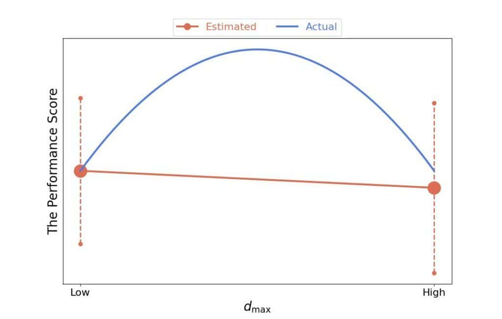
If our assumptions don’t hold, we may draw invalid conclusions. For instance, if we limit the model to linear main effects, we may conclude there’s no effect even though a quadratic relationship between and is strong:
Further, how to define an effect is still an open question in the statistical analysis of algorithms. Using differences in means as effects makes an implicit assumption that the mean values are representative of the distributions of . That may not be the case with every random forest and dataset.
We proposed determining based on the confidence interval width around a single mean. However, the confidence interval around the difference in means may have been more appropriate.
In our final model, and have fixed effects. That means that we shouldn’t generalize the conclusions to the ranges of values outside of those tested. If we want to do so, we should go with random-effects models. They treat the effects as random variables and allow extrapolation to unseen values.
We deliberately didn’t mention statistical significance, although it’s a common practice to conduct null-hypothesis significance tests (NHSTs). A growing body of literature criticizes the NHST framework. The main issue is that the subtleties of the NHST methods are prone to misinterpretation and confuse the majority of practitioners. That doesn’t mean that we shouldn’t use the NHSTs, but we should be careful and know what we’re doing.
Finally, we should keep in mind that fitting a forest may take a long time, so even if we go for a simpler model, estimating the effects could prove infeasible. In that case, we should reduce the size of the training set.
Here’s a quick list of steps to estimate the effects of and :
and to evaluate.
and ,  and
and  ).
). , we need values. or
  should suffice because higher-order effects are usually negligible.)., we minimize the width of the CIs around the means. and the number of trees in the design. We also visualize their confidence intervals.
We can vary some steps if we need, but the procedure to estimate the effects of and on a random forest’s performance will look more or less like the one above.
In this article, we presented a methodology for estimating how the depth and number of trees affect the performance of a random forest. We defined their hyper-parameters effects through differences in means, but there may be more appropriate effect definitions;;