Decision Tree vs. Naive Bayes Classifier | Baeldung on Computer Science

1. Overview

With machine learning dominating so many aspects of our lives, it’s only natural to want to learn more about the algorithms and techniques that form its foundation.

In this tutorial, we’ll be taking a look at two of the most well-known classifiers, Naive Bayes and Decision Trees.

After a brief review of their theoretical background and inner workings, we’ll discuss their strengths and weaknesses in a general classification setting. Finally, we’re going to talk about their suitability in applications.

2. Preliminaries

The techniques we’ll be talking about are, arguably, two of the most popular in machine learning. Their success stems from a combination of factors, including well established theoretical background, efficiency, scalability, and explainability.

However, they’re by no means perfect (as no technique ever is). In this article, we’ll be diving into the specifics of each technique and proceed to evaluate them comparatively.

To establish a common ground between the two, let’s first describe a general classification setting on which these methods can be applied. We are given a data set of $N$ entries, each one described by $M$ attributes, more commonly referred to as features. Each data entry is associated with a certain class, and this data will be used to determine the parameters of our classifier (training).

Because the ultimate goal of any machine learning algorithm is to generalize to data not seen during training, we always evaluate the accuracy of our model on a separate data set that was not used during training.

3. Naive Bayes

An extensive review of the Naive Bayes classifier is beyond the scope of this article, so we refer the reader to this article for more details. First, however, let us restate some of the background for the sake of completeness.

3.1. Background

The Naive Bayes classifier is a probabilistic model based on Bayes’ theorem which is used to calculate the probability $P(A|B)$ of an event $A$ occuring, when we are given some prior knowledge $B$ . The theorem can be expressed by a simple formula:

$P(A|B) = \frac{P(A,B)}{P(B)} = \frac{P(A) P(B|A)}{P(B)}$

Let’s configure this formula to fit our general classification setting. Our data entries $\hat{x} = (x_1, x_2, ..., x_M)$ correspond to one of $K$ classes $C_k, k \in \{1, 2, ..., K\}$ . We’re trying to estimate the probability $P(C_k | x_1, x_2, ..., x_M)$ of the entry belonging to class $C_k$ given the features $\hat{x}$ .

According to the thorem, this probabilty can be calculated as follows:

$P(C_k | \hat{x}) = \frac{P(C_k, \hat{x})}{P(\hat{x})} = \frac{P(C_k) P(\hat{x} | C_k)}{P(\hat{x})}$

The naïveté of this classifier stems from a core assumption that will significantly ease our calculations. All features $x_i$ are mutually independent. This means that we assume that each feature’s value does not influence other features’ values.

This assumption can now be included in our formula to obtain the final form of the equation.

$P(C_k | \hat{x}) = \frac{P(C_k, \hat{x})}{P(\hat{x})} = \frac{P(C_k) \prod_{i=1}^M P(x_i | C_k)}{P(\hat{x})}$

Remember that we’re trying to predict the correct class, not calculate the exact probabilities. We can therefore ignore the term $P(\hat{x})$ in the denominator, as it does not depend on the class.

Below we can see an example of how we calculate the individual components in the equation when we are given a data set of observations:

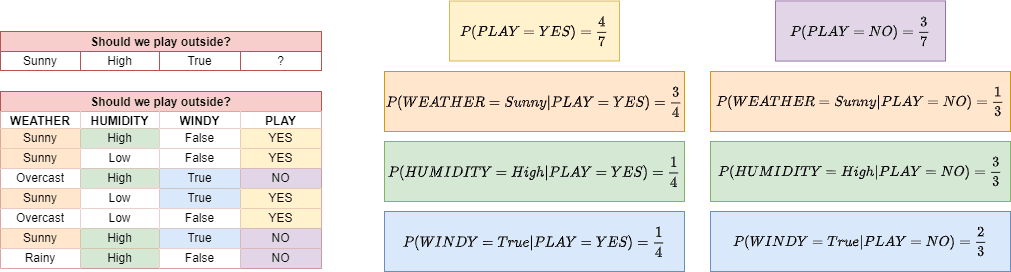
Along with the data set, we are also given a new observation, and we’re tasked to predict whether we should go outside and play.

In the case of discrete variables, evaluating each of the probabilities boils down to counting the number of samples in the data set that fit the criteria.

3.2. Comments

The benefits of the independence assumption are significant. It allows us to separate the features from each other and treat them as 1d distributions, which immensely reduces the number of computations, as well as reduces the required size of the data set.

Nevertheless, the assumption is quite bold and usually never holds in practice. This leads to inaccuracies in the calculations of the class probabilities. This would typically hinder its ability to classify correctly, but as a matter of fact, it usually doesn’t.

Enter the Maximum A Posteriori (MAP) estimator. The class with the highest posterior probability is elected as the output of the classifier. Inaccuracies in the probability calculation will not affect the outcome so long as the correct class’s posterior probability is higher than the others.

We can therefore infer that in the example above, we won’t go outside and play since the conditional probability $P(P=NO|\hat{x})$ is greater than $P(P=YES|\hat{x})$ . We welcome the reader to check that this inequality does indeed hold by taking the product of the individual probabilities and ignoring the denominator term.

3.3. Strengths and Weaknesses

A major advantage to Naive Bayes classifiers is that they are not prone to overfitting, thanks to the fact that they “ignore” irrelevant features. They are, however, prone to poisoning, a phenomenon that occurs when we are trying to predict a class $C_i$ but features uncommon to $C_i$ appear, causing a misclassification.

Naive Bayes classifiers are easily implemented and highly scalable, with a linear computational complexity with respect to the number of data entries.

Finally, it doesn’t require a lot of data entries to make proper classifications, although more data will result in more accurate calculations. Several improvements can be performed on this algorithm by further employing data preprocessing and statistical techniques.

Naive Bayes is strongly associated with text-based classification. Example applications include but are not limited to spam filtering and text categorization. This is because the presence of certain words is strongly linked to their respective categories, and thus the mutual independence assumption is stronger.

Unfortunately, several data sets require that some features are hand-picked before the classifier can work as intended.

4. Decision Trees

4.1. Background

Like the Naive Bayes classifier, decision trees require a state of $M$ attributes and output a decision. To clarify some confusion, “decisions” and “classes” are simply jargon used in different areas but are essentially the same.

A decision tree is formed by a collection of value checks on each feature. During inference, we check each individual feature and follow the branch that corresponds to its value. This traversal continues until a terminal node is reached, which contains a decision.

But how do we decide how the tree splits into branches and which features are used at each level? A simple approach would be to take every feature and form a branch for each possible value. This way, if the same data entry was encountered, it would lead to a correct decision.

However, such a model would not be able to generalize at all. To make matters worse, applying this method on a large data set would result in an enormous tree, adding to the computational requirements of the model.

A better idea would be to use the features in descending order of importance and even discard “useless” features that don’t increase accuracy. A commonly used metric to define the importance of a feature is the informational content. As defined mathematically by Shannon and Weaver, for a set of possible feature values $\{y_1, ..., y_k\}$ with associated probabilities $\{p(y_1), ..., p(y_k)\}$ , the information we get when the value is revealed is:

$I(p(y_1),...,p(y_k)) = \sum_{i=1}^k-p(y_i)\log_2p(y_i)$

Delving deeper into the math would be beyond the scope of this article. In short, when a feature’s values divide the data entries into approximately equal groups, then the informational content is higher, and the feature should be used early in the tree. This approach also has the benefit of creating relatively balanced decision trees. As a result, paths from the root to the terminal nodes are shorter, and therefore inference is faster.

A decision tree created using the data from the previous example can be seen below:

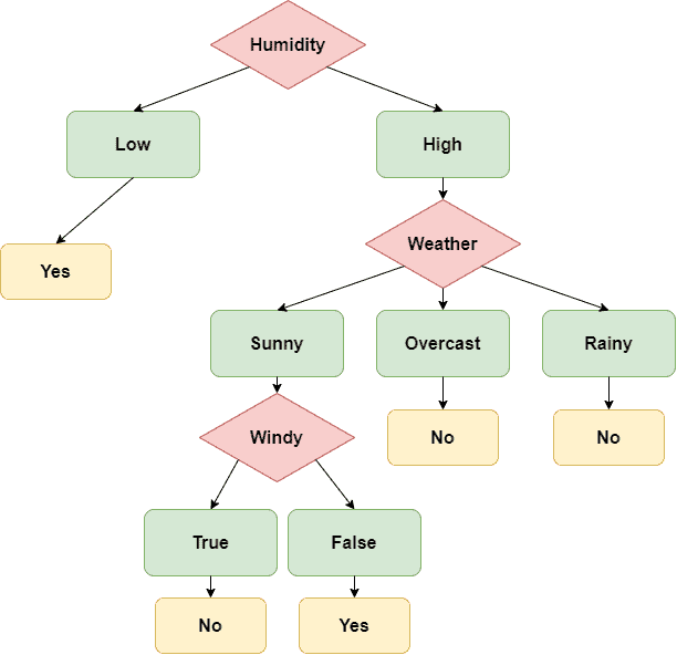
Given the new observation $(Sunny, High, True)$ , we traverse the decision tree and see that the output is $NO$ , a result that agrees with the decision made from the Naive Bayes classifier.

4.2. Strengths and Weaknesses

Probably the most significant advantage that Decision Trees offer is that of explainability. Their simple reasoning, along with their hierarchical structure, makes this an ideal candidate for usage, even by people unrelated to machine learning. A bonus that most machine learning methods lack is that decision trees can be easily visualized.

They are fast, efficient, and work with all kinds of data, both numerical and categorical, discrete or continuous. They can be set up effortlessly, requiring little to no data preprocessing. Additionally, the information-based heuristic used to determine the important features often reveals relationships within the data set that might not be visible at first glance.

However, unless properly pruned, decision trees tend to overfit the training data by eventually including unimportant or nonsense features. Data sets with uneven numbers of samples along each category will also lead to unbalanced trees or will lead to the pruning of features that are actually important.

Another disadvantage is that the algorithm separates the samples linearly. Imagine a continuous variable $x$ , a possible split would be $x=k$ . Depending on their nature, the data might not be linearly separable, and thus decision trees are unsuitable for these applications.

Despite their flaws, improved versions of decision trees such as random forests are very much used. A major application of Decision Trees and variants thereof lies in the business world for multifactorial decision making and risk assessment.

5. Comparison

Both methods we described perform very well on a variety of applications. But which one should you choose? Well, there are several things to consider regarding the nature of your data.

Are the features independent from each other? Do all features seem equally important, or do they have to be cherry-picked? In the former case, Naive Bayes is probably the better choice, while Decision Trees will most likely outperform it in the latter.

Are we trying to predict a class that appears very rarely in a data set? If that’s the case, it will likely be pruned out using the decision tree, and we won’t get the desirable results.

Fortunately, both methods are very fast, and in most cases, we will be able to test out both of them before deciding. It is important to note that for most problems out there, the methods will not be usable as-is but will probably require modifications and improvements.

6. Conclusion

We have delved into the specifics of the Naive Bayes and Decision Tree classifiers.

In summation, Naive Bayes’ independence assumption is a crucial factor for the classifier’s success. We have to make sure it applies (to some degree) to our data before we can properly utilize it.

Likewise, Decision Trees are dependent on proper pruning techniques so that overfitting can be avoided while keeping track of the classification objective.

All in all, they are both very useful methods and a great addition to our toolkit.

Full Archive

About Baeldung

Core Concepts

Operating Systems

Artificial Intelligence

Graph Theory

Latex