

Yes, we're now running our only Summer Sale. All Courses are 30% off until 20th July, 2026:
Learn through the super-clean Baeldung Pro experience:
>> Membership and Baeldung Pro.
No ads, dark-mode and 6 months free of IntelliJ Idea Ultimate to start with.
1. Overview
In this tutorial, we’ll study the similarities and differences between two well-loved algorithms in machine learning: support vector machines and neural networks.
We’ll start by briefly discussing their most peculiar characteristics, separately and individually. Then, we’ll list the similarities and differences between the two.
Lastly, we’ll study a few scenarios or use cases that require a decision between neural networks and support vector machines.
At the end of this article, we’ll know what distinguishes support vector machines from neural networks, and when to use one rather than the other.
2. Classification – a Problem of Boundary Detection
2.1. Classification in General
We’ll start this article by briefly discussing the problem of classification, that both support vector machines (hereafter: SVMs) and neural networks (NNs) help solve.
The problem of classification consists of the learning of a function of the form  , where
  is a feature vector and
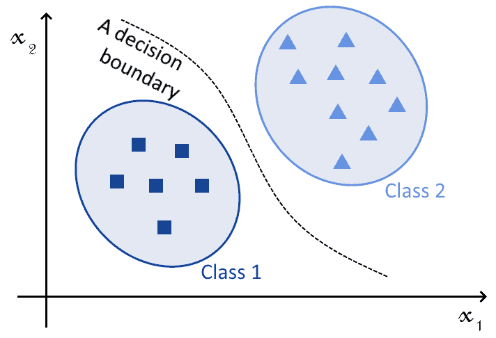
  is a vector corresponding to the classes associated with observations. This image represents classification in graphical form:
SVMs and NNs can both perform this task; with an appropriate choice of kernel, in the case of the SVM, or of activation function, in the case of NNs. The difference, therefore, isn’t in the types of tasks that they perform; but rather, in other characteristics of their theoretical bases and their implementation, as we’ll see shortly.
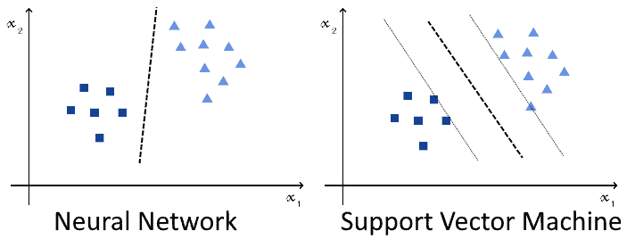
They both also can, which is equally important, approximate both linear and non-linear functions:
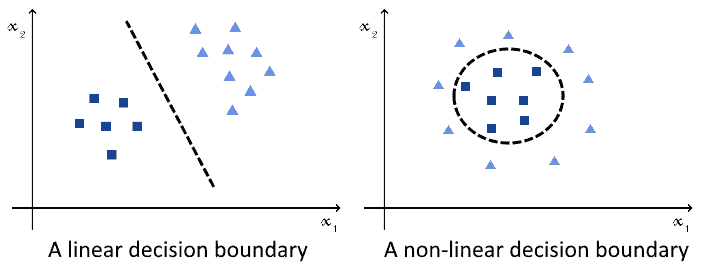
This means that both algorithms can equally tackle all types of classification problems; hence, the decision to use one over the other doesn’t depend on the problem itself.
One last note: both the SVMs and NNs that we discuss here refer exclusively to their variants for classification. These aren’t however the only possible forms of SVMs or NNs. If we’re interested in learning about their usage for regression, we can refer to our article on supervised learning for a discussion on those.
2.2. Approximating the Decision Boundary With NNs
Let’s start by considering neural networks and, in particular, single-layer networks. The universal approximation theorem tells us that a neural network with a single hidden layer and a non-linear activation can approximate, with an appropriate choice of weights, any continuous function.
If the decision boundary of a classification problem can be defined as a continuous function, which is always the case, then it can also be defined as a continuous mapping of the feature space. This, in turn, means that the universal approximation theorem guarantees that it can be approximated by a NN.
2.3. Approximating the Decision Boundary With SVMs
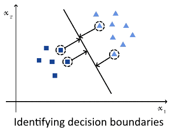
Regarding SVMs, though, the argument is a bit different. Support vector machines work by identifying the hyperplane that corresponds to the best possible separations among the closest observations belonging to distinct classes.
These observations take the name of “support vectors”; they are, for a properly-called SVM, a small subset of the whole training dataset. The SVM learns the hyperplane that best separates these support vectors, by means of maximization of the distance between these vectors and itself:
If the hyperplane or decision boundary doesn’t exist in the original feature space, then the SVM can project that space to a new vector space with higher dimensionality. The separation plane is then sought in the new, higher-dimensional vector space.
In the vector space where eventually the SVM finds a decision boundary, this decision boundary is a continuous region of that vector space. More specifically, it’s a hyperplane of that space. When projected onto the original feature space, the decision hyperplane then determines one or more continuous regions of the feature space.
The reason why the solution to a classification problem will always be found is that, as discussed here, SVMs aren’t restricted to the feature space in which the input is defined. Instead, they can increase the dimensionality of the problem up to a space in which a solution exists. This means, concretely, that they can use as many parameters as necessary until the size of the SVM allows the finding of a solution.
3. The Two Algorithms
3.1. SVMs for Classification
An SVM belongs to one of two types, and each of them behaves differently. These two types are the linear and the non-linear SVMs.
The linear SVM is the most simple, and it follows a simple rule. Whenever a dot product is computed between two features of its input, this product is equal to the linear combination of its input:

The non-linear SVM is, instead, an SVM for which this rule isn’t valid. When computing the output of the dot product between two features of the input, the non-linear SVM uses a kernel.
The word kernel, in machine learning, has a different meaning than that of kernels for operative systems. In artificial intelligence, a kernel corresponds to a method for the reduction in the dimensionality of the input to a classifier.
The kernel is, therefore, the function that’s used in place of a dot product between two vectors, whenever calculating one is needed. Examples of kernels include the polynomial kernel, the hyperbolic tangent, and the exponential kernel.
This means that an SVM can learn decision functions that have the shape, in some high-dimensionality space, of the kernel that it employs.
3.2. Neural Networks for Classification
Neural networks have a different way of operating and, in particular, don’t require kernels. This, of course, with the exception of convolutional neural networks.
A neural network for classification, in this context, correspond to a NN with a single hidden layer and a non-linear activation function. The most common types of non-linear activation functions for NNs for classification are:


All these functions take as an input a linear combination of a feature vector and a weight vector  . They then return an output that’s comprised in some finite interval, usually
  or
or  .
.
As mentioned before, a neural network with a single hidden layer and a non-linear activation function can approximate any given continuous function. If the decision boundary isn’t continuous in the original feature space, the addition of further layers in the NN can increase its dimensionality, up to a point in which it is. A deep neural network can, therefore, approximate all decision boundaries comprised of multiple continuous regions.
The problem, however, is that the universal approximation theorem includes no guarantee about the learnability of a decision function. This means that, for a given initial random configuration of the weights of the network, the NN may never learn the decision function through gradient descent. SVMs, on the other hand, always guarantee convergence.
4. Similarities Between SVMs and NNs
4.1. They Are Both Parametric
We can now list the similarities between the two algorithms, as we discussed them above.
The first similarity concerns the fact that both algorithms are parametric, though for different reasons. In the case of the SVM, the typical parameters are:
- the so-called soft-margin parameter, usually indicated with

- and the parameter of the kernel function usually called

Neural networks also use parameters, though they require significantly more of them. The most important parameters concern the number of layers and their size, but also the number of training epochs and the learning rate.
In this sense, the two models are similar insofar as they are both parametric, but dissimilar with regards to the type and number of parameters that they require.
4.2. They Can Both Embed Non-Linearity
Both machine learning algorithms embed non-linearity. This is done, in the case of SVMs, through the usage of a kernel method. Neural networks, instead, embed non-linearity by using non-linear activation functions. Both classes of algorithms can, therefore, approximate non-linear decision functions, though with different approaches.
In particular, the reason for the development of neural networks is exactly the necessity to overcome the problem of classification of non-linearly separable observations. This means that non-linearity is their fundamental raison d’être, and that their linear equivalent, such as convolutional neural networks that use ReLUs, were only developed later.
4.3. They Both Classify With Comparable Accuracy
Both SVMs and NNs can tackle the same problem of classification against the same dataset. This means that there’s no reason that derives from the characteristics of the problem for preferring one over the other.
What’s more important, though, is that they both perform with comparable accuracy against the same dataset, if given comparable training. If given as much training and computational power as possible, however, NNs tend to outperform SVMs.
As we’ll see in the next section, though, the time required to train the two algorithms is vastly different for the same dataset.
5. Differences Between the Two Approaches
5.1. Structure
We can now sum up the differences that we encountered when discussing the two algorithms independently.
The first difference concerns the underlying structure of the two algorithms. An SVM possesses a number of parameters that increase linearly with the linear increase in the size of the input. A NN, on the other hand, doesn’t.
Even though here we focused especially on single-layer networks, a neural network can have as many layers as we want. This, in turn, implies that a deep neural network with the same number of parameters as an SVM always has a higher complexity than the latter.
This is because of the more complex interaction between the model’s parameters. In NNs, this is limited to those belonging to adjacent layers. An SVM, instead, has parameters that all interact with one another.
5.2. Amount of Required Training Data
The second difference concerns the amount of information required to train the algorithm.
Support vector machines effectively use only a subset of a dataset as training data. This is because they reliably identify the decision boundary on the basis of the sole support vectors. As a consequence, for well-separated classes, the number of observations required to train an SVM isn’t high.
With regards to neural networks, instead, the training takes place on the basis of the batches of data that feed into it. This means that the specific decision boundary that the neural network learns is highly dependent on the order in which the batches of data are presented to it. This, in turn, requires processing the whole training dataset; or otherwise, the network may perform extremely poorly.
5.3. Training the Algorithm
One further difference relates to the time required to train the algorithm. SVMs are generally very fast to train, which is a consequence of the point we made in the previous section. The same is however not valid for neural networks.
As we discussed in our article on the advantages and disadvantages of neural networks, some particularly large NNs require in fact several days, sometimes weeks, in order to be trained. This means that restarting the training and initializing the random weights differently, for example, is possible for SVMs but very expensive for NNs.
5.4. Optimization of the Parameters
One further difference concerns the algorithm that neural networks and SVMs use in order to optimize their parameters. Typically, optimization for neural network takes place through gradient descent, as this is the most common technique. The usage of gradient descent is however also one of the reasons why neural networks sometimes can’t learn a function if their initial configuration places them at a function’s local minimum.
SVM use, instead, the method called quadratic programming. Quadratic programming consists of the optimization of a function according to linear constraints on its variables. Quadratic programming for SVMs is solved in practice with sequential minimal optimization, which allows the identification of a likely solution by iteratively computing the analytical solution to a subset of the problem.
5.5. Sensitivity to Initial Randomization of Weights
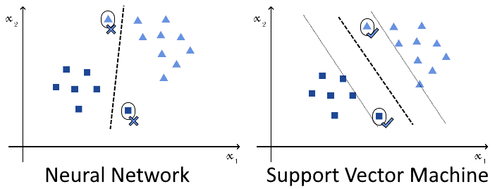
The last difference concerns a consequence of the different usage of optimization techniques. Because NNs use gradient descent, this makes them sensitive to the initial randomization of its weight matrix. This is because, if the initial randomization places the neural network close to a local minimum of the optimization function, the accuracy will never increase past a certain threshold:
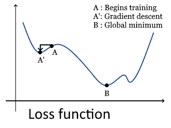
SVMs are more reliable instead, and they guarantee convergence to a global minimum regardless of their initial configuration.
6. Use Cases
We’re now going to see a brief discussion of three scenarios or case studies; this will help us understand how to choose one machine learning algorithm over the other in a concrete situation. All tasks can, in principle, be solved with both classes of algorithms. However, as we introduce constraints that have to do not quite with the machine learning task in itself, but rather with the process of developing a machine learning system, then one algorithm alone will be suitable to solve the particular problem along with its constraints.
6.1. The Feature Space Isn’t Sampled Thoroughly
We’re building a system for medical imaging for the detection of microcalcifications in tissues. We have reason to believe that the samples we collected are quite distant from any decision boundary that might distinguish between positive and negative samples. In other words, we believe that the training samples only represent instances of the two classes where most of the components of the input support the class affiliation.
As a consequence, after its deployment in the real world, we can expect the machine learning system to risk classifying incorrectly all observations that are closer to the opposite class than has ever been noted in training:
This system is going to have a predictable impact on the health of the population. For this reason, we’re concerned that it may incorrectly classify edge cases, and want to minimize this possibility.
We know that a neural network would certainly learn some decision function and perform well under training, testing, and validation. The function learned, however, isn’t necessarily distant from the observed samples. On the contrary, it may be very close to them, and thus incorrectly classify many future observations against real-world data:
In this case, the usage of SVMs may be preferable. This is because, as we discussed above, the SVM learns that decision boundary which maximizes the distance against the closest observations that belong to opposite classes. This, in turn, should produce better performances against the edge cases that we’re going to encounter in the future.
6.2. The Time for Training Is Scarce
In this second case, we’re working on a classifier for the detection, again, of medical diseases. This time the disease corresponds however to that of a newly-emerged pandemic, not to a problem that can be treated over extended periods. In this case, every day we can save before rolling-out the system leads to the saving of human lives.
We know that neural networks require significantly more time to train over a given dataset, with comparison to SVMs. Since, in this case, time is of the essence, our best bet is to use a support vector machine. Only after a first system is out, we could then consider developing one that requires significantly longer training time.
6.3. Any Marginal Increase in Accuracy Matters
In this last scenario, we’re building a system for driving autonomous vehicles. More specifically, we’re building a system for recognizing objects from the signal obtained by a lidar radar. The system we’re building requires the highest capacity to discriminate between objects; say, a pedestrian from a truck:
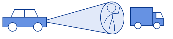
As a consequence, any little gain in accuracy is important. This also means that we can afford all the training data and computational time required to achieve the highest accuracy.
For this reason, in the case of autonomous driving, we may choose to use neural networks to build the classifier. This is, in fact, the common approach that scientists in machine learning apply today to autonomous vehicles.
Keep however in mind that this isn’t an absolute truth, and instances of usage of SVMs for autonomous driving also exist. Interestingly, SVMs in autonomous vehicles can also perform online evaluations on the effectiveness of neural networks.
7. Conclusions
In this article, we studied the main similarities and differences between support vector machines and neural networks.
We started by discussing the problem of classification in general, and its relationship with machine learning. We then studied, separately, the way in which SVMs and NNs help solve this problem.
Then, we listed the primary similarities and differences between the two algorithms for the solution of classification tasks.
Lastly, we used this newly acquired knowledge in practical cases. Specifically, we used it to identify the most suitable algorithm for the solution of three learning scenarios.