Yes, we're now running our only Summer Sale. All Courses are 30% off until 20th July, 2026:
Introduction to the Classification Model Evaluation
Last updated: February 28, 2025

Learn through the super-clean Baeldung Pro experience:
>> Membership and Baeldung Pro.
No ads, dark-mode and 6 months free of IntelliJ Idea Ultimate to start with.
1. Introduction
In machine learning, classification refers to predicting the label of an observation. In this tutorial, we’ll discuss how to measure the success of a classifier for both binary and multiclass classification problems. We’ll cover some of the most widely used classification measures; namely, accuracy, precision, recall, F-1 Score, ROC curve, and AUC.
We’ll also compare two most confused metrics; precision and recall.
2. Binary Classification
Binary classification is a subset of classification problems, where we only have two possible labels. Generally speaking, a yes/no question or a setting with 0-1 outcome can be modeled as a binary classification problem. For instance, a well-known problem is predicting whether an e-mail is spam or not.
Given two classes, we can talk in terms of positive and negative samples. In this case, we say a given e-mail is spam (positive) or not spam (negative).
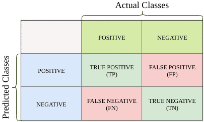
For a given sample observation, the actual class is either positive or negative. Similarly, the predicted class is also either positive or negative. We can visualize the outcome of a binary classification model using a confusion matrix, like the one presented above.
There are four categories associated with the actual and predicted class of an observation:
- True Positive (
 ): Both the actual and predicted values of the given observation are positive.
 - False Positive (
 ): The given observation is negative but the predicted value is positive.
 - True Negative (
 ): Both the actual and predicted values of the given observation are negative.
 - False Negative (
 ): The given observation is predicted to be negative, despite, in fact, being positive.
The diagonal of the confusion matrix presents the correct predictions. Obviously, we want the majority of our predictions to reside here.
FPs and FNs are classification errors. In statistics, FPs are referred to as Type I errors, and FNs are referred to as Type II errors. In some cases, Type II errors are dangerous and not tolerable.
For example, if our classifier is predicting if there is a fire in the house, a Type I error is a false alarm.
On the other hand, a Type II error means that the house is burning down and the fire department isn’t aware.
3. Binary Classification Measures
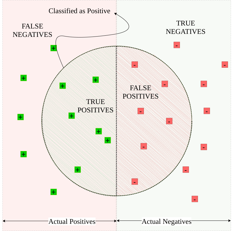
Suppose we have a simple binary classification case as shown in the figure below. The actual positive and negative samples are distributed on rectangular surfaces.
However, our classifier marks the samples inside the circle as positive and the rest as negative.
How did our classifier do?
Many metrics are proposed and being used to evaluate the performance of a classifier. Depending on the problem and goal, we must select the relevant metric to observe and report.
In this section, we’ll try to understand what do some popular classification measures represent and which one to use for different problems.
3.1. Accuracy
The most simple and straightforward classification metric is accuracy. Accuracy measures the fraction of correctly classified observations. The formula is:
![\[\textrm{Accuracy} = \frac{TP + TN}{\textrm{\# samples}} = \frac{TP + TN}{TP + TN + FP + FN}\]](/wp-content/ql-cache/quicklatex.com-6d680a76ee4c1a72fafb29bf74907470_l3.svg "Rendered by QuickLaTeX.com")
Thinking in terms of the confusion matrix, we sometimes say “the diagonal over all samples”. Simply put, it measures the absence of error rate. An accuracy of 90% means that out of 100 observations, 90 samples are classified correctly.
Although 90% accuracy sounds very promising at first, using the accuracy measure in imbalanced datasets might be misleading.
Again recall the spam e-mail example. Consider out of every 100 e-mails received, 90 of them are spam. In this case, labeling each e-mail as spam would lead to 90% accuracy with an empty inbox. Think about all the important e-mails we might be missing.
Similarly, in the case of fraud detection, only a tiny fraction of transactions are fraudulent. If our classifier were to mark every single case as not fraudulent, we’d still have close to 100% accuracy.
3.2. Precision and Recall
An alternative measure to accuracy is precision. Precision is the fraction of instances marked as positive that are actually positive. In other words, precision measures “how useful are the results of our classifier”. The mathematical notation is:
![\[\textrm{Precision} = \frac{TP}{TP + FP}\]](/wp-content/ql-cache/quicklatex.com-b9ba417e2c0ac23ef425618e4d1cf4ca_l3.svg "Rendered by QuickLaTeX.com")
Otherwise speaking, a precision of 90% would mean when our classifier marks an e-mail as spam, it is indeed spam 90 out of 100 times.
Another way to look at the TPs is by using recall. Recall is the fraction of true positive instances that are marked to be positive. It measures “how complete the results are” — that is, which percentage of true positives are predicted as positive. The representation is:
![\[\textrm{Recall} = \frac{TP}{TP + FN}\]](/wp-content/ql-cache/quicklatex.com-416875633d5577634fc2aa1b7eb2ffe8_l3.svg "Rendered by QuickLaTeX.com")
That is to say, a recall of 90% would mean that the classifier correctly labels 90% of all the spam e-mails, hence 10% are marked as not spam.
Classical classifiers have a threshold value, for which they mark the lower results as negative and higher results as positive. Changing the defined threshold value for a binary classifier leads to changes in the predicted labels. So, reducing the rate of one error type leads to an increase in the other one. As a result, there is a trade-off between precision and recall.
All in all, both precision and recall measure the absence of errors in special terms. Perfect precision is equivalent to no FPs (no Type I errors), while on the other hand, perfect recall means there are no FNs (no Type II errors). In some cases, we need to select the relevant error type to consider, depending on the problem goal.
3.3. F-1 Score
Usually, having a balanced recall and precision is more important than having one type of error really low. That’s why generally we take both precision and recall into consideration. Several classification measures are developed to identify this problem.
For example, the F-1 score is the harmonic mean of precision and recall. It gives equal importance to Type I and Type II errors. The calculation is:
![\[\textrm{F-1 Score} = \frac{2 \times \textrm{Precision} \times \textrm{Recall}}{\textrm{Precision} + \textrm{Recall}}\]](/wp-content/ql-cache/quicklatex.com-427c003face698912b8b5493c4b1cfa2_l3.svg "Rendered by QuickLaTeX.com")
When the dataset labels are evenly distributed, accuracy gives meaningful results. But if the dataset is imbalanced, like the spam e-mail example, we should prefer the F-1 score.
Another point to keep in mind is; accuracy gives more importance to TPs and TNs. On the other hand, the F-1 score considers FN and FPs.
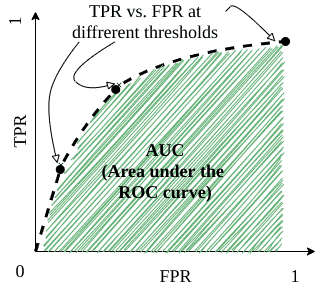
3.4. ROC Curve and AUC
A well-known method to visualize the classification performance is a ROC curve (receiver operating characteristic curve). The plot shows the classifier’s success for different threshold values.
In order to plot the ROC curve, we need to calculate the True Positive Rate ( ) and the False Positive Rate (
 ), where:
![\[TPR = \frac{TP}{TP + FN}\]](/wp-content/ql-cache/quicklatex.com-65ce573832125d372b9aab6909b3751c_l3.svg "Rendered by QuickLaTeX.com")
![\[FPR = \frac{FP}{FP + TN}\]](/wp-content/ql-cache/quicklatex.com-420f5f4c938289ca7760bd4e89c23e9a_l3.svg "Rendered by QuickLaTeX.com")
To better understand what this graph stands for, first imagine setting the classifier threshold to  . This will lead to labeling every observation as positive. Thus, we can conclude that lowering the threshold marks more items as positive. Having more observations classified as positive results in having more TPs and FPs.
Conversely, setting the threshold value to  causes every observation to be marked as negative. Then, the algorithm will label more observations as negative. So, increasing the threshold value will cause both TP and FP numbers to decrease, leading to lower TPR and FPR.
For each different threshold value, we get different TP and FP rates. Plotting the result gives us the ROC curve. But how does the ROC curve help us find out the success of a classifier?
In this case, AUC helps us. It stands for “area under the curve”. Simply put, AUC is the area under the ROC curve. In case we have a better classification for each threshold value, the area grows. A perfect classification leads to an AUC of 1.0.
On the contrary, worse classifier performance reduces the area. AUC is often used as a classifier comparison metric for machine learning problems.
4. Multi-Class Classification
When there are more than two labels available for a classification problem, we call it multiclass classification. Measuring the performance of a multiclass classifier is very similar to the binary case.
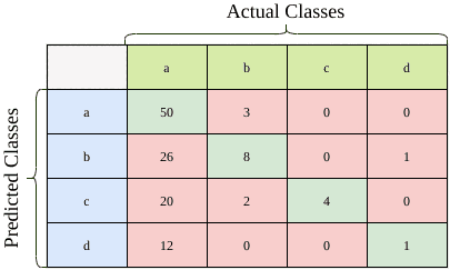
Suppose a certain classifier generates the confusion matrix presented above. There are 127 samples in total. Now let’s see how well the classifier performed.
Recall that accuracy is the percentage of correctly classified samples, which reside on the diagonal. To calculate accuracy, we need to just divide the number of correctly classified samples by the total number of samples.
![\[\textrm{Accuracy} = \frac{\textrm{\# correctly classified}}{\textrm{\# samples}} = \frac{50 + 8 + 4 + 1}{127} = \frac{63}{127} = 49.6\%\]](/wp-content/ql-cache/quicklatex.com-8479b0a0f965f5713d20efa8da2a6266_l3.svg "Rendered by QuickLaTeX.com")
So, the classifier correctly classified almost half of the samples. Given we have five labels, it is much better than the random case.
Calculating the precision and recall is a little trickier than the binary class case. We can’t talk about the overall precision or recall of a classifier for multiclass classification. Instead, we calculate precision and recall for each class separately.
Class by class, we can categorize each element into one of TP, TN, FP, or FN. Hence, we can rewrite the precision formula as:
![\[\textrm{Precision}(class=a)} = \frac{TP\textrm{ for class a}}{\textrm{\# classified as class a}} = \frac{TP(class=a)}{TP(class=a) + FP(class=a)} = \frac{50}{53} = 94.3\%\]](/wp-content/ql-cache/quicklatex.com-d756ba299b6b2d397df029a92d0686cf_l3.svg "Rendered by QuickLaTeX.com")
Similarly, the recall formula can be rewritten as:
![\[\textrm{Recall}(class=a) = \frac{TP\textrm{ for class a}}{\textrm{\# actual class a}} = \frac{TP(class=a)}{TP(class=a) + FN(class=a)} = \frac{50}{108} = 46.3\%\]](/wp-content/ql-cache/quicklatex.com-1a1f57b588a245a08fa1a38c26127f1f_l3.svg "Rendered by QuickLaTeX.com")
Correspondingly, we can calculate precision and recall values for other classes.
![\[\begin{aligned} \textrm{Precision}(class=b)} & = \frac{8}{35} & \textrm{Recall}(class=b) & = \frac{8}{13} \\ \textrm{Precision}(class=c)} & = \frac{4}{26}$ & \textrm{Recall}(class=c) & = \frac{4}{4} \\ \textrm{Precision}(class=d)} & = \frac{1}{13} & \textrm{Recall}(class=d) & = \frac{1}{2} \end{aligned}\]](/wp-content/ql-cache/quicklatex.com-28df5243ba97d408dbbcfff8e6469ecc_l3.svg "Rendered by QuickLaTeX.com")
5. Conclusion
In this tutorial, we have investigated how to evaluate a classifier depending on the problem domain and dataset label distribution. Then, starting with accuracy, precision, and recall, we have covered some of the most well-known performance measures.
Precision and recall are two crucial metrics, each minimizing a different type of statistical error. F-1 Score is another metric for measuring classifier success, and it considers both Type I and Type II errors.
We have briefly explained the ROC curve and AUC measure to compare classifiers. Before concluding, we have discussed some differences between binary and multiclass classification problems and how to adapt the elementary metrics to the multiclass case.