

Yes, we're now running our only Summer Sale. All Courses are 30% off until 20th July, 2026:
How to Improve Naive Bayes Classification Performance?
Last updated: February 13, 2025
Learn through the super-clean Baeldung Pro experience:
>> Membership and Baeldung Pro.
No ads, dark-mode and 6 months free of IntelliJ Idea Ultimate to start with.
1. Introduction
Classification is a type of supervised machine learning problem, where we assign class labels to observations. In this tutorial, we’ll learn about a fast and simple classification method: the Naive Bayes classifier.
Naive Bayes classifier is especially known to perform well on text classification problems. Some widely adopted use cases include spam e-mail filtering and fraud detection. The baseline of spam filtering is tied to the Naive Bayes algorithm, starting from the 1990s. As another example, we can utilize a Naive Bayes classifier to guess if a sentence in an unknown language talks about animals or not.
First of all, we’ll investigate the theory behind this classifier and understand how it works. After grasping the basics, we’ll explore ways to improve the classification performance.
2. Naive Bayes Classifier
Naive Bayesian classifier inputs discrete variables and outputs a probability score for each candidate class. The predicted class label is the class label with the highest probability score.
It determines the class label probabilities based on the observed attributes. Each feature is assumed to be independent. Class label probability scores are calculated by Bayes’ Law:
![\[P(C|A) = \frac{P(A \cap C)}{P(A)} = \frac{P(A |C) P(C)}{P(A)}\]](/wp-content/ql-cache/quicklatex.com-ffa73ba3ebf9ce85365e956e31d36999_l3.svg "Rendered by QuickLaTeX.com")
Technically, the Bayes’ Law calculates the conditional probability  , representing the probability of
  given that
  is observed. In this formula, represents the class label from a set of available
  classes, and represents an observation with
  attributes:
![\[A = {a_1, a_2, ..., a_m}\]](/wp-content/ql-cache/quicklatex.com-c064a922eedd2750e571f8936651bf6b_l3.svg "Rendered by QuickLaTeX.com")
So, for each observation , we’ll to compute probabilities for each class label  :
:
![\[P(C_i |A) = \frac{P(a_1,a_2,...,a_m|C_i) P(C_i)}{P(a_1,a_2,...,a_m)}\]](/wp-content/ql-cache/quicklatex.com-5cb31e53780f558b0eb5e45b3b68864b_l3.svg "Rendered by QuickLaTeX.com")
Only then can we decide on the predicted class  , with the largest probability score
  . We’ll apply the following tricks to simplify the calculations:
- Since each attribute is conditionally independent, we can directly multiply conditional probabilities of distinct attributes:
![\[P(a_1,a_2,...,a_m|C_i) = \prod_{j=1}^{m} P(a_j|C_i)\]](/wp-content/ql-cache/quicklatex.com-6944b71da4d33fb903b66706ae3729ce_l3.svg "Rendered by QuickLaTeX.com")
- The probability
 in the denominator part is constant. Hence, we can ignore it when comparing the scores for different classes.
As a result, we can compare the output of the simplified formula to decide on the class label:
![\[P(C_i |A) \propto \Big ( \prod_{j=1}^{m}P(a_j|C_i) \Big ) P(C_i)\]](/wp-content/ql-cache/quicklatex.com-85a1961b13dda0f9d8abaf9c33e6a6a0_l3.svg "Rendered by QuickLaTeX.com")
The class  with the maximum probability is chosen to be the predicted class. In other words, we say observation belongs to class .
The validity of the formula we use to compute the class probabilities relies on the conditional independence assumption. If two features encode the same information, the Naive Bayes classifier will double-count their effect and reach a wrong conclusion.
Another implicit assumption comes with the Naive Bayes classifier. The algorithm doesn’t treat features differently. So, all features have an equal effect on the result. Sometimes this assumption leads to over-simplification.
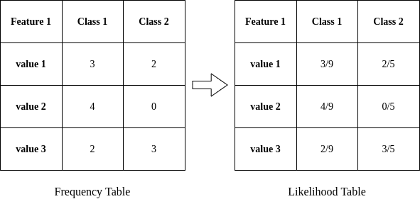
In practice, we train a model by extracting statistics from the training set. Utilizing a frequency table and a likelihood table for each feature in the calculations facilitates the process:
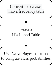
A frequency table derived from the observations includes possible feature values grouped together. The likelihood table contains the probability values instead of the number of occurrences for different classes. Using these tables, we decide on an observation’s class by multiplication and comparison operations:
3. Ways to Improve Naive Bayes Classification Performance
The Naive Bayes classifier model performance can be calculated by the hold-out method or cross-validation depending on the dataset. We can evaluate the model performance with a suitable metric. In this section, we present some methods to increase the Naive Bayes classifier model performance:
| Improve Performance | Won’t Improve |
|---|---|
| Remove correlated features | Hyper-parameter tuning |
| Use log probabilities in calculations | Handling missing values |
| Eliminate the zero observations | Training with more data |
| Handle continuous variables | Dimension reduction |
| Handle text data | Early Stopping |
| Re-train the model with new data | Applying ensemble methods |
| Parallelize calculations |
We need to keep in mind that Naive Bayes is a very simple yet elegant classification algorithm. Some common methods don’t work in the Naive Bayes case.
For instance, one of the first methods that come to mind is to tune the hyper-parameters of the model. However, the Naive Bayes classifier has a very limited parameter set. Depending on the implementation, sometimes the number of classes is the only parameter, which in practice, we have no control on. So, hyper-parameter tuning is not a valid method to improve Naive Bayes classifier accuracy.
Like all machine learning algorithms, we can boost the Naive Bayes classifier by applying some simple techniques to the dataset, like data preprocessing and feature selection.
One major data preprocessing step is handling missing values. How we handle the missing data is a major decision for most models. Though, the Naive Bayes classifier is immune to missing values. We can just ignore them because the algorithm handles the input features separately at both model construction and prediction phases.
3.1. Remove Correlated Features
As we already mentioned, the highly correlated features are counted twice in the model. Double counting leads to overestimating the importance of those features. So, the performance of the Naive Bayes classifier degrades.
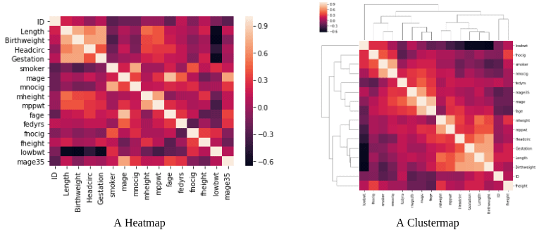
We need to eliminate correlated features and adhere to the assumption of independent features. To detect and eliminate them, we can use a correlation matrix to compare feature pairs.
Alternatively, we can perform feature selection based on probability. We can explore the combined probabilities of different features, and try to understand their prediction power on the output variable.
In Python, we can use the Seaborn library to plot correlation heatmaps and clustermaps. Assuming our data resides in a data frame df:
import seaborn as sns

# calculate the correlations
correlations = df.corr()

# plot the heatmap
sns.heatmap(correlations, xticklabels=correlations.columns, yticklabels=correlations.columns, annot=True)

# plot the clustermap
sns.clustermap(correlations, xticklabels=correlations.columns, yticklabels=correlations.columns, annot=True)
Heatmap is a common tool that we use to visualize the feature correlation matrix. The clustermap shows the correlations as a hierarchically-clustered heatmap. Hence, reading the clustermap to eliminate correlated features is easier:
3.2. Use Log Probabilities
Multiplying very small numbers will lead to even smaller numbers. It is difficult to precisely store and compare these very small numbers. We face these problems when working with probability values.
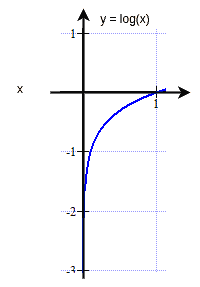
To avoid working with very small numbers, we can work within the log probability space by taking the logarithm of probability values.
The log function maps the probability values from [0, 1] range to the (-  , 0] range. Thus, the log probability values will be negative. The smaller the actual probability value is, it’ll be mapped to a larger negative value by the log function:
We need to remember that multiplication operation becomes an addition in the logarithm space. So, taking the logarithm of the whole equation gives us:
![\[log \big ( P(C_i |A) \big ) \propto \Big ( \sum_{j=1}^{m} log \big ( P(a_j|C_i) \big ) \Big ) log \big ( P(C_i) \big )\]](/wp-content/ql-cache/quicklatex.com-79a4276da956a0ad0d7335fb9de68c01_l3.svg "Rendered by QuickLaTeX.com")
This mapping approach works because to classify in Naive Bayes, we need to know which class has the largest probability rather than what the specific probability is. Taking the logarithm will not change the ordering of class label probability scores. Hence, we can still decide which class has the highest probability.
3.3. Eliminate the Zero Observations Problem
If the training data has a different frequency distribution compared to the test set, the Naive Bayes classifier performs poorly. The classifier is especially affected by values not being represented in the training set.
If the model comes across a categorical feature that isn’t present in the training set, the probability of 0 is assigned to that new category. This is very dangerous, as multiplying 0 with other features’ probabilities will result in 0.
Even when we use the log probabilities, the zero observation problem exists. Because  , and summation with will cancel out all the valid information from other features.
We need to check for these cases and take action if the test data set has zero frequency issues. The most known approach is to use Laplace Smoothing. In this technique, we add a parameter to both numerator and denominator when calculating the class probabilities.
For example, we can add a smoothing parameter (of 1) when calculating the class probabilities:
![\[P(C|A) = \frac{P(A |C) P(C) + 1}{P(A) + 1}\]](/wp-content/ql-cache/quicklatex.com-ba441d816d1680d9b75d6d51d60d5df0_l3.svg "Rendered by QuickLaTeX.com")
The smoothing parameter ensures that the probability value is never zero. Applying a smoothing technique assigns a very small probability estimate to such zero frequency occurrences, hence, regularize the Naive Bayes classifier.
3.4. Handle Continuous Variables
We’ve covered how to calculate the probability values for categorical features. But, counting the number of occurrences equal to some value doesn’t work for real numbers.
An easy method to represent real numbers as categories is discretization. We map intervals to category labels. This way, we have labels representing different ranges. Then we use these labels as categories and calculate the probabilities accordingly.
Some Naive Bayes implementations assume Gaussian distribution on continuous variables. Thus, the Naive Bayes classifier uses probabilities from a z-table derived from the mean and standard deviation of the observations. In this case, it’s a good idea to check the distribution of any numerical variable and handle them accordingly.
If a continuous feature doesn’t follow the normal distribution, we can use non-parametric methods like kernel density estimation to have a more realistic estimate of the probability density function. We don’t need to limit ourselves to the normal distribution. Instead, we need to represent the features appropriately.
3.5. Handle Text Data
Text datasets require special preprocessing steps. Removing stop words, normalizing the words by switching to lower case, and applying stemming or lemmatization are common techniques.
Creating word embeddings helps us understand which words are used together or occur in the same context. Utilizing word2vec or another embedding algorithm leads to better representation of words with vectors.
Following the best practices in handling words and documents helps us boost the performance of our machine learning model.
3.6. Re-Train the Model
For some complex machine learning algorithms, training the model from scratch takes a very long time. As a result, some alternative methods are proposed to update the model, like online training. Re-training the model often requires a lot of resources.
However, as new data is accumulated, we might need to re-train a model:
- Training with a larger dataset ensures better model generalization
- The trend of data changes in a dynamic environment
- New patterns can form in an adversarial environment
Contrary to most algorithms, it is very fast to re-train the Naive Bayes model. The algorithm is computationally efficient. It easily handles high-dimensional data without being affected by the curse of dimensionality. Categorical features with high-cardinality don’t add to computational complexity, as well. As a result, the Naive Bayes classifier performs faster than alternative classification methods.
We can easily reconstruct the model as new data becomes available. This way, we can detect shifts or drifts in the dataset. As a result, we guarantee that the performance of the model will not degrade as time passes.
3.7. Parallelize Probability Calculations
When building a Naive Bayes classification model, we can gain additional performance by using parallelized computations.
The probabilities of each attribute can be calculated independently due to the independence assumption. So, we calculate the probabilities of each feature separately. Dividing the work leads to the speedup of calculations and enables us to handle large datasets more easily.
3.8. Usage with Small Datasets
The Naive Bayes classifier denies the existence of any relationship between input features. Thus, it only models the relationship between an input feature and the output class label. The hypothesis function is simpler compared to other more complex algorithms. As a result, the training phase requires less data.
Furthermore, it is less likely to overfit with limited data. Since the model omits any interaction between features, it is far from creating a high variance model. Conversely, it suffers from high bias.
3.9. Ensemble Methods
Ensemble learning proved to increase performance. Common ensemble methods of bagging, boosting, and stacking combine results of multiple models to generate another result. The main point of ensembling the results is to reduce variance.
However, we already know that the Naive Bayes classifier exhibits low variance. So, mixing it with other classifiers doesn’t help. There’s no need to try ensemble methods to boost classifier accuracy.
3.10. Usage as a Generative Model
Generative models have the ability to generate new data instances. For example, generative adversarial networks (GAN) are proven useful for synthetic dataset generation. Given a dataset, it generates new data points following the original distribution.
Naive Bayes is a generative model, as well. It learns the classes based on the characterization of data distribution. We can use this model to create a new fictitious dataset following the same probability distribution.
4. Conclusion
In this article, we investigated the Naive Bayes classifier, which is a very robust and easy to implement machine learning algorithm.
We began with the probabilistic fundamentals making it work. Then we had a deeper look at how we can train and use the algorithm in practice. Finally, we’ve investigated ways to improve the classification performance.
To sum up, we’ve seen that some common practices to improve the classifier performance won’t work with the Naive Bayes classifier. The probabilistic approach has different challenges, requiring special handling. Nevertheless, we can apply the methods discussed in this article to overcome possible performance issues.