Correlated Features and Classification Accuracy

1. Introduction

In this tutorial, we’ll analyze the implication of the correlation phenomenon into machine learning algorithms, such as classification algorithms.

The discussion that follows applies to the problem of pattern recognition in general.

2. Interlude: Correlazione and Causality

Correlation doesn’t imply causality. For example, the increase in the wind causes an increase in the speed of the blades in a wind farm, which leads to an increase in the production of electricity, but the increase in the speed of the blades doesn’t cause an increase in the wind. However, the two phenomena are related in that we can predict the numerical value of one from the numerical value of the other.

The following figure illustrates another point of view on the same example:

From an epistemological point of view, the two concepts are logically distinct: the correlation is symmetric (variable $A$ correlated to variable $B$ implies that variable $B$ is correlated to variable $A$ ), while causality is asymmetric, as we have seen in the example just done.

Correlation is a concept that we can analyze from a statistical point of view. Given the statistical nature of most methods in machine learning, it, therefore, makes sense to speak, in general, of correlation but not of causality.

There is an excellent discussion of these concepts in our tutorial on what the correlation coefficient actually represents.

The phenomena of correlation don’t influence the structure and way of working of a classifier. However, they have a negative influence on individual predictions, which can impact the quality of the final results.

The reason lies, as we’ll see, in some generic constraints that arise when analyzing a problem with an algorithm. Of these constraints, the most important is the size of the available dataset.

3. Correlation and Collinearity

Correlation and collinearity are different phenomena, but they have points of contact, so we’ll consider them as examples of correlation.

Correlation can be positive if the increase of one variable is related to the increase of another variable, or negative if the increase of one variable is related to the decrease of the other variable.

3.1. Correlation

In statistics, correlation is a measure of the degree of dependence (as we have seen, not necessarily causal) between two random variables. In general, the word correlation implies a linear relationship.

Correlation can be a positive phenomenon, as it can make it possible to make predictions on one variable knowing the values of another variable.

Correlation is synonymous with dependence, so two independent random variables from a statistical point of view are not correlated.

There are several measures of correlation, known as correlation coefficients (typically denoted by $\rho$ or $r$ ). The most common is the Pearson correlation coefficient, which measures the degree of linear dependence between two variables. This linear relationship can have sense even if the mathematical dependence between the two variables follows a non-linear function.

The are other correlation coefficients, also sensitive to non-linear relationships, such as Spearman’s rank correlation and Mutual Information.

3.2. Correlation Coefficients

The Pearson product-moment correlation coefficient (PPMCC), also known as Pearson’s correlation coefficient or simply correlation coefficient, is a measure of the quality of least-squares fitting to the original data. Mathematically, it is the ratio between the covariance, $\Sigma$ , of the two variables and their standard deviations $\sigma (X)$ , $\sigma (Y)$ :

$\rho_{XY}=\frac{\Sigma_{XY}}{\sigma(X)\sigma(Y)}=\frac{\mathrm{E}\left[(X-\mu_{X})(Y-\mu_{Y})\right]}{\sigma(X)\sigma(Y)}=\frac{\mathrm{E}\left[XY\right]-\mathrm{E}[X]\mathrm{E}[Y]}{\sqrt{\mathrm{E}[X^{2}]-\mathrm{E}[X]^{2}}\sqrt{\mathrm{E}[Y^{2}]-\mathrm{E}[Y]^{2}}}$

where, for a dataset with $N$ records and means $\mu$ :

$\Sigma_{XY}=\frac{1}{N}\sum_{i=1}^{N}(x_{i}-\mu_{X})(y_{i}-\mu_{Y})$

Without referring to means, we can express it in an equivalent way as:

$\mathbf{\Sigma}_{XY}=\frac{1}{2n^{2}}\sum_{i}^{N}\sum_{j=i}^{N}(x_{i}-x_{j})(y_{i}-y_{j})=\frac{1}{n^{2}}\sum_{i}^{N}\sum_{j>i}^{N}(x_{i}-x_{j})(y_{i}-y_{j})$

3.3. Collinearity

In statistics, collinearity (also multicollinearity) is a phenomenon in which one predictor variable in a multiple regression model can be linearly predicted from the others with a substantial degree of accuracy.

Multicollinearity does not reduce the predictive power or reliability of the model as a whole, at least within the sample data set; it only affects calculations regarding individual predictors. That is, a multivariate regression model with collinear predictors can indicate how well the entire bundle of predictors predicts the outcome variable, but it may not give valid results about any individual predictor, or about the redundancy between predictors.

No multicollinearity usually refers to the absence of perfect multicollinearity, which is an exact (non-stochastic) linear relation among the predictors.

For a general linear model:

$y=\beta\mathbf{X}+\epsilon$

reorganizing the matrix form of this expression, we can write the statistical predictor:

$\hat{\beta}=\left(\mathbf{X}^{\mathrm{T}}\mathbf{X}\right)^{-1}\mathbf{X}^{\mathrm{T}}y$

However, in the case of collinearity, we can’t compute the inverse. Therefore, this predictor does not exist. It is worth understanding why.

3.4. Problems with Collinearity

We focus our attention on square matrices, which are the only ones for which we can compute the inverse. Product $\mathbf{X}^{\mathrm{T}}\mathbf{X}$ is a square matrix.

The rank of a square matrix is the number of linearly independent rows or columns. A full-rank matrix has a number of linearly independent rows or columns equal to the number of rows or columns of the matrix, otherwise, it is called rank-deficient and in this case, for a matrix $\mathbf {A}$ ( $N \times N$ ), we have $\mathrm {rank} ( \mathbf {A}) <N$ .

For non-square matrices, the rank is the minimum between rows and columns. In general, the input matrix for a dataset will be full-rank if all columns (features) are independent.

In the presence of collinearity (perfect multicollinearity), we have, thus, data matrices rank-deficient.

Two fundamental results of algebra establish:

$rank(\mathbf{A})=rank(\mathbf{A}^{T}\mathbf{A})=rank(\mathbf{A}\mathbf{A}^{\mathrm{T}})$
$\det (\mathbf{A})=0$ if $\mathbf{A}$ is rank-deficient

In the case of our predictor, if a generic non-square matrix $\mathbf{X}$ result from a dataset is rank-deficient, thus the square matrix $\mathbf{X}^{\mathrm{T}}\mathbf{X}$ is rank-deficient and its determinant is null.

For a $2 \times 2$ matrix, the inverse can be calculated according to the expression:

$\mathbf{{A}}=\left(\begin{array}{cc} a & b\\ c & d \end{array}\right)$

$\mathbf{A}^{-1}=\frac{1}{ad-bc}\left(\begin{array}{cc} d & -b\\ -c & a \end{array}\right)$

But $ad-bc = \det (\mathbf {A})$ . From this result and the two previous properties it follows that in the case of collinearity, a linear predictor does not exist. This result is generalizable to matrices of any order.

Multicollinearity is a characteristic of the data matrix, not the underlying statistical model.

4. The Curse of Dimensionality

The number of records in the dataset conditions the maximum number of features that we can deal with in a statistical model. In certain situations, it may be necessary to apply some preprocessing technique, to transform the dataset into an equivalent dataset that offers greater guarantees of obtaining good results.

Let us consider as an example a typographic character recognition system whose purpose is to achieve the best possible classification starting from a series of images.

The first step is to identify some features (feature extraction), that is some input parameters that we can link to the category predicted by the classifier to which each image belongs.

We can intuitively agree that increasing the number of features increases the performance of the classifier. In this case, what we’re doing is increasing the information entering the system, which leads in principle to the possibility of recognizing patterns with higher resolution, and thus improving the mapping between inputs and outputs.

This situation suggests arbitrarily increase the number of features, for example by identifying each input of our system with a single pixel of the image, obtaining an input dimension of the order of thousands or tens of thousands.

However, empirical practice shows that increasing the number of features beyond a certain limit worsens the performance of the classifier. Let’s see why.

4.1. An Example

We divide each variable into a certain number of intervals. This splits the entire input space into several cells, as in the following figure:

Each instance of the dataset corresponds to a point in one of the cells, and a value of the output variable $y$ .

Given a new point in the input space, we can determine the corresponding $y$ value by calculating all points in the dataset that belong to the same cell as the given point and averaging the values of $y$ .

Increasing the number of subdivisions increases the resolution of the system at the cost of exponentially increasing the number of cells. If each input variable is divided into $M$ ranges and the dimension of the input is $D$ , then the total number of cells is equal to $M ^ {D}$ .

The quality of our classifier gets worse when we increase $D$ beyond a certain limit because we arrive at the situation of having cells inside which there are no representative points of the dataset. This aberration is known as the “curse of dimensionality”, and in this case, the only solutions are to increase the number of records in the dataset or decrease the number of features.

However, for real problems where the dataset is usually given by a series of measurements, the number of records is fixed when we build our classifier. In practice, the size of the dataset conditions the maximum number of features that we can “solve” within our system.

Correlation and collinearity, although phenomena that do not globally affect the performance of our classifier, are negative elements from a practical point of view. In these cases, we have redundant data that could lead our classifier to have to work with a number of features beyond the intrinsic resolving capacity of the dataset.

The rule is, therefore, to perform a preprocessing of the dataset to obtain, in a controlled and reproducible way, the least number of features containing most of the original information, where the variance of the data is a measure of this amount of information.

This is exactly what the Principal Component Analysis does.

5. Principal Component Analysis (PCA)

Correlation and collinearity of the input matrix are to be considered aberrations. They introduce redundant information that can lead, as we have seen in the extreme case of the images of the previous section, to the situation of having an insufficient amount of data to have adequate resolving power in all regions of the input space.

Let’s formalize the problems we have discussed. We call $\mathbf {X}$ the input matrix of our dataset, formed by $D$ features (columns) and $N$ rows (records of the dataset). In the case of correlations in the input we have the following problems:

In the process of building our classifier, we need to identify the features on which the mapping between input and output depends. Not having a model in general, the choice of the features is partly arbitrary and introduces, in general, correlations in the dataset
In this case, $\mathbf {X}$ could be rank-deficient if not all components are linearly independent
It’s a good thing to have features with high variance since they will be more informative and more important
It’s a bad thing to have highly correlated features, or high covariance, since they can be deduced from one another with little loss in information, and thus keeping them together is redundant. In this case, the choice of the number of features may be excessive for the capabilities offered by the number of data available

What we’re looking for is a way of:

Transform the original $\mathbf {X}$ input matrix into a new full-rank $\mathbf {X} '$ matrix, if possible. This solves most of the problems related to correlation and collinearity
Identify a criterion that allows reducing the size of the input in a controlled way, eliminating information that is not essential for the mapping between input and output

The PCA solves these problems. It is a rotation and a projection of the original data on a new set of linearly independent axes, equal in number to the number of features. The result is, in an ideal situation, a new full-rank data matrix. This new matrix becomes the new dataset, smaller than the original one, where the number of features retains an arbitrary amount of information of the original data.

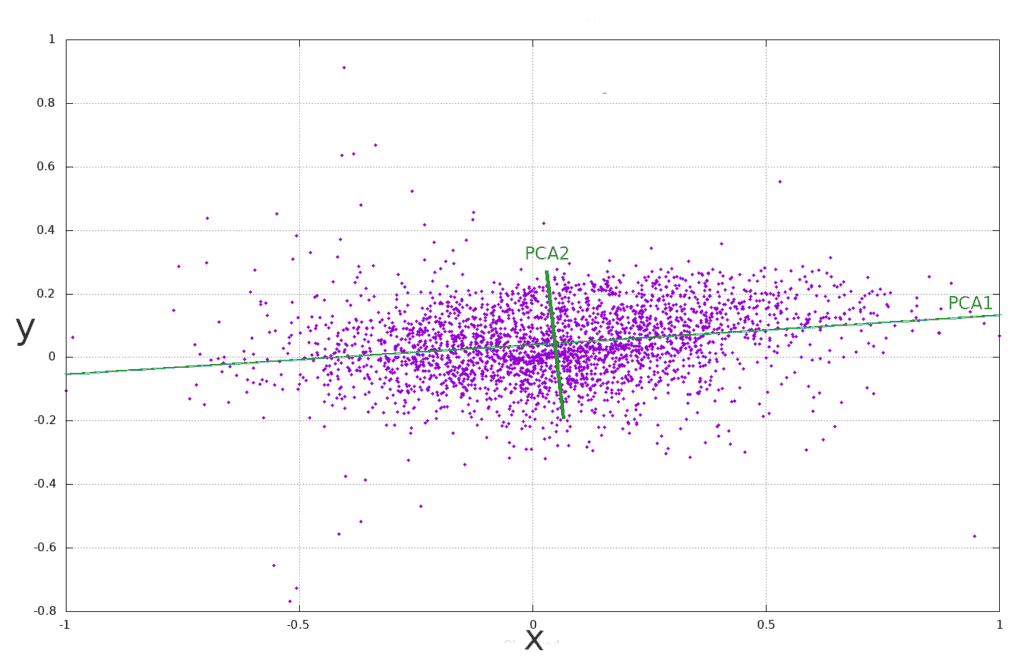
The following image illustrates the rotation and projection of the original axes $(x, y)$ into a new set of orthogonal axes PCA1 and PCA2:

A detailed exposition of the PCA can be found in our tutorial on PCA: Principal Component Analysis.

6. Conclusion

In this tutorial, we have analyzed how correlation phenomena are generally harmful within a predictive method.

The fixed size of the dataset conditions the maximum amount of features that we can incorporate into the algorithm. In the case of correlation effects, the data contains redundant information. In this situation, we can reduce the size of the dataset in a controlled manner, eliminating some of the redundant information.

The Principal Component Analysis is one of the methodologies used for this purpose and forms part of the arsenal of techniques of obligatory knowledge for every technician in machine learning.

Full Archive

About Baeldung

Core Concepts

Operating Systems

Artificial Intelligence

Graph Theory

Latex