

Yes, we're now running our only Summer Sale. All Courses are 30% off until 20th July, 2026:
Underfitting and Overfitting in Machine Learning
Last updated: February 28, 2025
Learn through the super-clean Baeldung Pro experience:
>> Membership and Baeldung Pro.
No ads, dark-mode and 6 months free of IntelliJ Idea Ultimate to start with.
1. Introduction
In machine learning, we aim to build predictive models that forecast the outcome for a given input data. To achieve this, we take additional steps to tune the trained model. So, we evaluate the performance of several candidate models to choose the best-performing one.
However, deciding on the best-performing model is not a straightforward task because selecting the model with the highest accuracy doesn’t guarantee it’ll generate error-free results in the future. Hence, we apply train-test splits and cross-validation to estimate the model’s performance on unseen data.
In this tutorial, we’ll focus on two terms in machine learning: overfitting and underfitting. These terms define a model’s ability to capture the relationship between input and output data. Both of them are possible causes of poor model performance.
2. What Are Underfitting and Overfitting
Overfitting happens when we train a machine learning model too much tuned to the training set. As a result, the model learns the training data too well, but it can’t generate good predictions for unseen data. An overfitted model produces low accuracy results for data points unseen in training, hence, leads to non-optimal decisions.
A model unable to produce sensible results on new data is also called “not able to generalize.” In this case, the model is too complex, and the patterns existing in the dataset are not well represented. Such a model with high variance overfits.
Overfitting models produce good predictions for data points in the training set but perform poorly on new samples.
Underfitting occurs when the machine learning model is not well-tuned to the training set. The resulting model is not capturing the relationship between input and output well enough. Therefore, it doesn’t produce accurate predictions, even for the training dataset. Resultingly, an underfitted model generates poor results that lead to high-error decisions, like an overfitted model.
An underfitted model is not complex enough to recognize the patterns in the dataset. Usually, it has a high bias towards one output value. This is because it considers the variations of the input data as noise and generates similar outputs regardless of the given input.
When training a model, we want it to fit well to the training data. Still, we want it to generalize and generate accurate predictions for unseen data, as well. As a result, we don’t want the resulting model to be on any extreme.
Let’s consider we have a dataset residing on an S-shaped curve such as a logarithmic curve. Fitting a high-order parabola passing through the known points with zero error is always possible. On the other hand, we can fit a straight line with a high error rate.
The first solution generates an overly complex model and models the implicit noise as well as the dataset. As a result, we can expect a high error for a new data point on the original S-shaped curve.
Conversely, the second model is far too simple to capture the relationship between the input and output. Hence, it will perform poorly on new data, too:
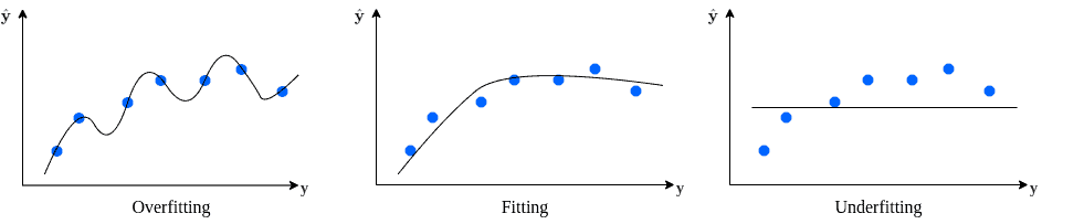
Reducing the error from overfitting or underfitting is referred to as the bias-variance tradeoff. We aim to find a good fitting model in between.
3. How to Detect Underfitting and Overfitting?
The cause for overfitting is a misinterpretation of training data. So, the model produces less accurate results for unseen data. However, an overfitted model generates very high accuracy scores during the training phase.
Similarly, underfitted models don’t effectively capture the relationship between the input and output data because it is too simple. As a result, the underfitted model performs poorly, even with the training data.
If the data scientist is not careful, they can easily be mistaken and deploy an overfitted model into production. Though, applying the decisions of an overfitted model’s predictions will result in errors. For example, the business may lose value or come face to face with dissatisfied customers.
Deploying an underfitting model into production may hurt business as it generates inaccurate results. Thus, shaping decisions upon erroneous outputs leads to unreliable business decisions, as well.
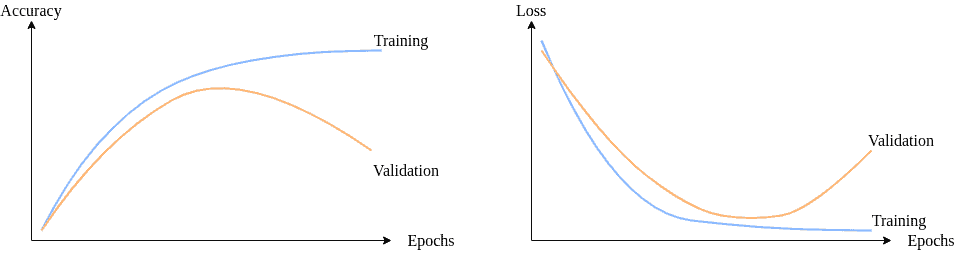
We need to closely watch model loss and accuracy to decide how the model is fitted to the dataset:
3.1. Detecting Overfitting
We can detect overfitting in different steps in the machine learning life cycle using various techniques. Adopting the holdout method and saving a portion of the dataset for testing is crucial.
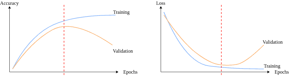
To determine when overfitting begins, we plot training error and validation error together. As we train the model, we expect both to decrease at the beginning. However, after some point, the validation error would increase, whereas the training error keeps dropping. Training further after this point leads to overfitting:
3.2. Detecting Underfitting
Usually, detecting underfitting is more straightforward than detecting overfitting. Even without using a test set, we can decide if the model is performing poorly on the training set or not. If the model accuracy is insufficient on the training data, it has high bias and hence, underfitting.
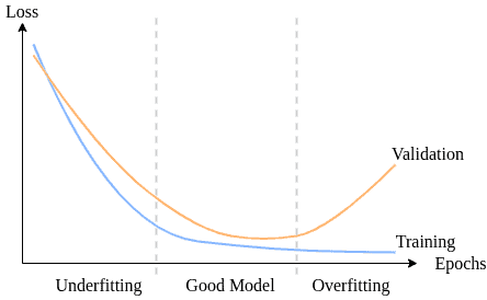
A challenge in machine learning is to decide the model complexity as we don’t know the underlying optimal complexity of the dataset. Moreover, we have incomplete information regarding the environment, and the data we have contains noise.
Under these circumstances, we need to overcome the bias-variance tradeoff to fit a model:
4. How to Cure Underfitting and Overfitting
We have already discussed what overfitting and underfitting in machine learning are and how we can detect them. Now, let’s try to understand what are our options to combat them:
4.1. Cures for Overfitting
If the model is overfitting, the most sensible approach is to reduce model complexity. This way, we can enable it to generalize better.
In an attempt to reduce model flexibility, we can reduce the number of input features. To enable fewer feature combinations within the model, we can either manually select which features to keep or take advantage of a feature selection algorithm.
Alternatively, we can apply regularization to suppress higher-order terms in our model. So, we keep all the features but limit the magnitude of their feature importance in the outcome. As expected, regularization works well with a lot of features that contain slightly helpful information.
For instance, adding a dropout layer in neural networks is a form of regularization. Moreover, we can set a regularization term to limit the weights of a neural network.
Early stopping is another type of regularization we can utilize for iterative models. The main idea is to stop model training when specific criteria are satisfied, such as when validation accuracy starts to decrease.
Another possible approach to model fitting is to use more training examples to train the model to generalize better.
4.2. Cures for Underfitting
To prevent underfitting, we need to ensure the model complexity.
The first method that comes to mind is to obtain more training data. However, this is not an easy task for most problems. In such cases, we can bring data augmentation into service. So, we can increase the amount of data available by creating slightly modified synthetic copies of the data points at hand.
Similarly, increasing the number of passes on the training data is a viable approach for iterative algorithms. Increasing the number of epochs in a neural network is a well-known practice to ensure model fitting.
Another way to increase model complexity is to increase the size and number of model parameters. We can introduce engineered features from the dataset. For example, a product of numerical features or n parameter of n-grams generates new features.
Alternatively, we can reduce regularization. Some implementations implicitly include default regularization parameters to overfitting. Checking the default parameters is a good start point. As we’re trying to get out of a limited feature set, there’s no need to introduce limiting terms into the model.
Replacing the approach is another solution. For example, the selection of the kernel function in SVM determines the model complexity. Thus, the choice of kernel function might lead to overfitting or underfitting.
5. Summary
Let’s summarize what we’ve discussed so far in a comparison table:
| Overfitting | Underfitting |
|---|---|
| Model is too complex | Model is not complex enough |
| Accurate for training set | Not accurate for training set |
| Not accurate for validation set | Not accurate for validation set |
| Need to reduce complexity | Need to increase complexity |
| Reduce number of features | Increase number of features |
| Apply regularization | Reduce regularization |
| Reduce training | Increase training |
| Add training examples | Add training examples |
6. Conclusion
In this article, we examined overfitting and underfitting in machine learning.
Firstly, we’ve discussed the meaning of the terms and their relation to model complexity. Then, we’ve considered possible ways to detect overfitting and underfitting, including plotting loss and accuracy curves. Afterward, we’ve learned about different methods to prevent fitting problems. Lastly, we concluded with a summary.