

Learn through the super-clean Baeldung Pro experience:
>> Membership and Baeldung Pro.
No ads, dark-mode and 6 months free of IntelliJ Idea Ultimate to start with.
Last updated: February 28, 2025
Learn through the super-clean Baeldung Pro experience:
>> Membership and Baeldung Pro.
No ads, dark-mode and 6 months free of IntelliJ Idea Ultimate to start with.
In this tutorial, we’ll introduce the multiclass classification using Support Vector Machines (SVM). We’ll first see the definitions of classification, multiclass classification, and SVM. Then we’ll discuss how SVM is applied for the multiclass classification problem. Finally, we’ll look at Python code for multiclass classification using Scikitlean SVM.
In artificial intelligence and machine learning, classification refers to the machine’s ability to assign the instances to their correct groups.
For example, in computer vision, the machine can decide whether an image contains a cat or a dog, or if an image contains a human body or not. In Natural Language Processing (NLP), the machine can tell the sentiment of a given text whether it’s positive, negative, or neutral.
For the machine to be able to decide how to assign an instance to its group, it has to learn the patterns of that assignment from the training features available in a labeled training data set.
We’ve two types of classification: binary classification and multiclass classification.
In this type, the machine should classify an instance as only one of two classes; yes/no, 1/0, or true/false.
The classification question in this type is always in the form of yes/no. For example, does this image contain a human? Does this text has a positive sentiment? Will the price of a particular stock increase in the next month?
In this type, the machine should classify an instance as only one of three classes or more.
The following are examples of multiclass classification:
SVM is a supervised machine learning algorithm that helps in classification or regression problems. It aims to find an optimal boundary between the possible outputs.
Simply put, SVM does complex data transformations depending on the selected kernel function and based on that transformations, it tries to maximize the separation boundaries between your data points depending on the labels or classes you’ve defined.
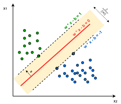
In the base form, linear separation, SVM tries to find a line that maximizes the separation between a two-class data set of 2-dimensional space points. To generalize, the objective is to find a hyperplane that maximizes the separation of the data points to their potential classes in an  -dimensional space. The data points with the minimum distance to the hyperplane (closest points) are called Support Vectors.
In the image below, the Support Vectors are the 3 points (2 blue and 1 green) laying on the scattered lines, and the separation hyperplane is the solid red line:
The computations of data points separation depend on a kernel function. There are different kernel functions: Linear, Polynomial, Gaussian, Radial Basis Function (RBF), and Sigmoid. Simply put, these functions determine the smoothness and efficiency of class separation, and playing around with their hyperparameters may lead to overfitting or underfitting.
In its most simple type, SVM doesn’t support multiclass classification natively. It supports binary classification and separating data points into two classes. For multiclass classification, the same principle is utilized after breaking down the multiclassification problem into multiple binary classification problems.
The idea is to map data points to high dimensional space to gain mutual linear separation between every two classes. This is called a One-to-One approach, which breaks down the multiclass problem into multiple binary classification problems. A binary classifier per each pair of classes.
Another approach one can use is One-to-Rest. In that approach, the breakdown is set to a binary classifier per each class.
A single SVM does binary classification and can differentiate between two classes. So that, according to the two breakdown approaches, to classify data points from  classes data set:
 SVMs. Each SVM would predict membership in one of the classes.
 SVMs.
SVMs.Let’s take an example of 3 classes classification problem; green, red, and blue, as the following image:
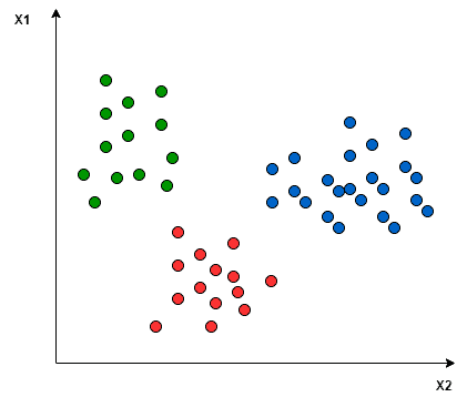
Applying the two approaches to this data set results in the followings:
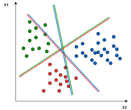
In the One-to-One approach, we need a hyperplane to separate between every two classes, neglecting the points of the third class. This means the separation takes into account only the points of the two classes in the current split. For example, the red-blue line tries to maximize the separation only between blue and red points. It has nothing to do with green points:
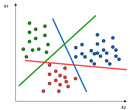
In the One-to-Rest approach, we need a hyperplane to separate between a class and all others at once. This means the separation takes all points into account, dividing them into two groups; a group for the class points and a group for all other points. For example, the green line tries to maximize the separation between green points and all other points at once:
One of the most common real-world problems for multiclass classification using SVM is text classification. For example, classifying news articles, tweets, or scientific papers.
The following Python code shows an implementation for building (training and testing) a multiclass classifier (3 classes), using Python 3.7 and Scikitlean library.
We developed two different classifiers to show the usage of two different kernel functions; Polynomial and RBF. The code also calculates the accuracy and f1 scores to show the performance difference between the two selected kernel functions on the same data set.
In this code, we use the Iris flower data set. That data set contains three classes of 50 instances each, where each class refers to a type of Iris plant.
We’ll start our script by importing the needed classes:
from sklearn import svm, datasets
import sklearn.model_selection as model_selection
from sklearn.metrics import accuracy_score
from sklearn.metrics import f1_score
Load Iris data set from Scikitlearn, no need to download it separately:
iris = datasets.load_iris()
Now we need to separate features set  from the target column (class label)
  , and divide the data set to 80% for training, and 20% for testing:
X = iris.data[:, :2]
y = iris.target
X_train, X_test, y_train, y_test = model_selection.train_test_split(X, y, train_size=0.80, test_size=0.20, random_state=101)
We’ll create two objects from SVM, to create two different classifiers; one with Polynomial kernel, and another one with RBF kernel:
rbf = svm.SVC(kernel='rbf', gamma=0.5, C=0.1).fit(X_train, y_train)
poly = svm.SVC(kernel='poly', degree=3, C=1).fit(X_train, y_train)
To calculate the efficiency of the two models, we’ll test the two classifiers using the test data set:
poly_pred = poly.predict(X_test)
rbf_pred = rbf.predict(X_test)
Finally, we’ll calculate the accuracy and f1 scores for SVM with Polynomial kernel:
poly_accuracy = accuracy_score(y_test, poly_pred)
poly_f1 = f1_score(y_test, poly_pred, average='weighted')
print('Accuracy (Polynomial Kernel): ', "%.2f" % (poly_accuracy*100))
print('F1 (Polynomial Kernel): ', "%.2f" % (poly_f1*100))
In the same way, the accuracy and f1 scores for SVM with RBF kernel:
rbf_accuracy = accuracy_score(y_test, rbf_pred)
rbf_f1 = f1_score(y_test, rbf_pred, average='weighted')
print('Accuracy (RBF Kernel): ', "%.2f" % (rbf_accuracy*100))
print('F1 (RBF Kernel): ', "%.2f" % (rbf_f1*100))
That code will print the following results:
Accuracy (Polynomial Kernel): 70.00
F1 (Polynomial Kernel): 69.67
Accuracy (RBF Kernel): 76.67
F1 (RBF Kernel): 76.36
Out of the known metrics for validating machine learning models, we choose Accuracy and F1 as they are the most used in supervised machine learning.
For the accuracy score, it shows the percentage of the true positive and true negative to all data points. So, it’s useful when the data set is balanced.
For the f1 score, it calculates the harmonic mean between precision and recall, and both depend on the false positive and false negative. So, it’s useful to calculate the f1 score when the data set isn’t balanced.
Playing around with SVM hyperparameters, like C, gamma, and degree in the previous code snippet will display different results. As we can see, in this problem, SVM with RBF kernel function is outperforming SVM with Polynomial kernel function.
In this tutorial, we showed the general definition of classification in machine learning and the difference between binary and multiclass classification. Then we showed the Support Vector Machines algorithm, how does it work, and how it’s applied to the multiclass classification problem. Finally, we implemented a Python code for two SVM classifiers with two different kernels; Polynomial and RBF.