

Learn through the super-clean Baeldung Pro experience:
>> Membership and Baeldung Pro.
No ads, dark-mode and 6 months free of IntelliJ Idea Ultimate to start with.
Last updated: February 13, 2025
Learn through the super-clean Baeldung Pro experience:
>> Membership and Baeldung Pro.
No ads, dark-mode and 6 months free of IntelliJ Idea Ultimate to start with.
In this tutorial, we’ll study the advantages and disadvantages of artificial neural networks (ANNs) in comparison to support vector machines (SVMs).
We’ll first start with a quick refresh on their structure. Then, we’ll identify what pros and cons they possess according to the theory.
Finally, we’ll test a neural network model and a support vector machine against the same benchmark datasets.
At the end of this tutorial, we’ll know why we should use neural networks instead of support vector machines and vice-versa.
In our article on the differences between support vector machines and neural networks, we discussed how the two architectures for the respective machine learning models are built. Here, we focus on the identification and testing of the specific advantages and disadvantages that the two models have when solving concrete machine learning tasks.
In general, in the literature on machine learning feedforward neural networks and support vector machines are used almost interchangeably. However, at a more advanced level, we can state that some important differences do indeed exist.
This is because the two architectures correspond perfectly only in a limited selection of cases, and in particular, when we discuss linear SVMs. In other cases, for non-linear SVMs and ANNs, the difference becomes more significant as the complexity of the problem increases. A skilled data scientist should therefore know which model to prefer, in order to squeeze that extra performance from his machine learning systems.
A feedforward neural network is a parametric model that consists of  vectors of weights
  , of
, of  activation functions
  , and of an input vector
  . The neural network is thus a model that computes an output
  from as:

The input vector also takes the name of the input layer for the neural network. The pairs that include the activation function  together with its associated parameters
  , for
, for  , take instead the name of hidden layers. Finally, the last pair
  is the output layer for that model.
Schematically, we can represent the graph of a neural network as a directed weighted graph:
The support vector machine is instead a non-parametric machine learning model that comprises of a kernel function and a decision hyperplane. A hyperplane in -dimensional space is defined by a set of parameters plus a bias term, corresponding to the coefficients for each of the components of any vector in that space.
If a decision hyperplane doesn’t exist in the vector space with dimensionality  , corresponding to the feature plus label space, the SVM projects all observations to a new vector space
  and searches there for a suitable decision hyperplane. If there’s no hyperplane there either, it keeps increasing the dimensionality of
  until it finds one.
In this sense, the SVM guarantees eventual convergence and therefore the identification of some solutions to its problem. Because the solution isn’t guaranteed to have a certain dimensionality, though, this makes the SVM a non-parametric model.
We can aprioristically identify some advantages and disadvantages that, in general, should characterize ANNs in comparison to SVMs, regardless of the specific nature of the task that they have to perform.
The first is that we can aprioristically constrain the size of a network and its number of layers. This means that we can help solve the curse of dimensionality for machine learning models by arbitrarily imposing a certain limit on the network size.
SVMs with non-linear kernels can’t do that. Instead, the number of their parameters increases linearly with the number of support vectors that they employ. In some cases, especially when we’re working with text data, the SVM may end up employing several thousand support vectors.
The second advantage is the general rapidity of neural networks in performing predictions after training. This is because a neural network needs to only compute as many weight matrix multiplications and activation functions as there are layers. Matrix multiplications are typical tasks for parallelization, and therefore can be computed rapidly.
ANNs also have theoretical disadvantages, though, with comparison to SVMs. The first disadvantage consists of longer training time for neural networks. This is because the very first decision hyperplane in an SVM is guaranteed to be located between support vectors belonging to different classes. Neural networks don’t offer this guarantee and, instead, position the initial decision function randomly.
The second disadvantage consists in the non-guaranteed convergence of neural networks. By an appropriate choice of hyperparameters, a neural network can approach a target function until a satisfactory result is reached; however, SVMs are theoretically grounded in their capacity to converge to the solution for a problem.
The third disadvantage lies in the parametric and fixed size of the neural network. Earlier, we considered this an advantage of the network; however, if a real-world problem is characterized by a higher degree of complexity than was observable during training, the fixed size of the neural network implies that the network will learn a solution that represents the training observations, but may not generalize well to previously unseen data.
The last disadvantage consists of the scarce human interpretability of the neural networks when compared with SVMs. This is because the decision function of an SVM is known to be equally distant to the classes observed during training, while the neural network might learn a decision function that gets arbitrarily close to one of the two classes.
These theoretical advantages, however, refer to the two models in abstract terms, but may not be valid for all particular datasets. For this reason, we now set forth and test these expectations by comparing the two machine learning models against the same benchmark problems.
We can now empirically evaluate whether the theoretical expectations that we hold are verified with respect to some specific datasets. For this section, we use as benchmarks three datasets, and we compare the performances of the two model architectures:
The metrics according to which we compare the two models are:
In both cases, the shorter the time, the better it is.
We aren’t, in this case, interested in comparing them against criteria of accuracy or loss, as we normally would otherwise. This is because we’d need to tinker with the hyperparameters of the two models and consider several options for them. This, in turn, would increase the complexity of the comparison between the models without adding much to our understanding of their advantages.
Instead, we train them until convergence over the full dataset and measure the time it takes to conduct training and prediction.
Finally, for the replicability of the experiments, we can state that all tests were done with the Python implementations of both ANNs and SVMs.
This first example is a trivial dataset that we use as a lower bound for the complexity of the problem, which the two models have to solve. This is because we can aprioristically predict the characteristics of the neural network model that learns the solution, and we can, therefore, easily test it against the SVM.
This problem is the XOR classification task:
 |
 |
|
|---|---|---|
| 0 | 0 | 0 |
| 0 | 1 | 1 |
| 1 | 0 | 1 |
| 1 | 1 | 0 |
We can implement this problem, in practice, by creating 1000 copies of all possible values for the components of the input vector. The neural network that solves this problem has an input with two components, a hidden layer with two nodes, and an output layer:
We trained the neural network by imposing an early interruption in the training process in case of early convergence, which it reached after around 50 iterations. The support vector machine, instead, decided by itself the correct number of parameters for the solution to this problem and continued training until convergence.
We obtained these results:
| Model | Training time | Prediction time |
|---|---|---|
| ANN | 1.4711 | 0.0020 |
| SVM | 0.0190 | 0.0069 |
This experiment confirms the expectation that the training time for ANNs is longer than the training time for SVMs. On the other hand, it shows that prediction time is shorter in ANNs than in SVMs.
The second experiment consists of the classification of the flowers contained in the Iris dataset. This problem is generally suitable for multiclass classification, but we can decrease its dimensionality to a binary classification task in order to constrain its complexity. We can do this by mapping one of the three classes to  , and the other two classes to
  .
.
Then, we can train the models to recognize the distinction between these binary classes:
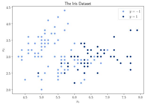
For this problem, because we don’t have good theoretical guidance on the neural network architecture that should solve this task, we test a neural network with two hidden layers and two neurons each. It appears, in fact, that the observations constitute slightly separated regions of the 2D plane, and, as we studied in our article on hidden layers, we should therefore try to use two hidden layers.
We replicated the dataset 100 times and fed it to the classifiers. Upon convergence, we obtained the following results:
| Model | Training time | Prediction time |
|---|---|---|
| ANN | 12.7850 | 0.0050 |
| SVM | 7.9350 | 3.7296 |
This experiment, too, confirms the rapidity of the SVM during the training phase and its slowness during prediction, with comparison to the neural network.
Finally, we can compare the performances of the two models in the multiclass classification problem of the digits in the MNIST dataset:
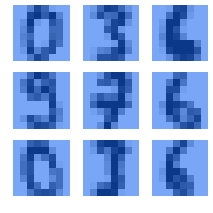
For this dataset, we use a neural network architecture that comprises two hidden layers with 48 and 36 neurons. The particular version of the dataset that we use has observations with 64 features and ten classes. Therefore, it makes sense to use a number  of hidden neurons per layer comprised between the size of the input and that of the output, as
  .
.
Both models converge, and as they do, we obtain the following results:
| Model | Training time | Prediction time |
|---|---|---|
| ANN | 7.4254 | 0.0011 |
| SVM | 1.1048 | 0.5199 |
It appears, therefore, that for multiclass classification tasks, too, the performances of neural networks and support vector machines conform to the theoretical expectation.
From this, we can conclude that the theoretical predictions are confirmed. ANNs outperformed SVMs in all benchmark datasets with regards to prediction time and underperformed in regards to training time. We can therefore formulate a criterion for determining when to use one over the other:
We can now ask ourselves, in what concrete cases might we have to apply the criterion that we just learned. That is, in what case saving training time or prediction time might make such a difference that it may actually mandate the choice of one model over the other. This has to do with the development and operational requirements that we have to fulfill when we build our machine learning model, but also with the expected usage of the system that we’re creating.
The first example corresponds to a situation in which we have to cover the burden of training the model ourselves, either financially or with computational time. But, after deployment, we can outsource to a third party the cost of prediction.
If, for example, we’re a small laboratory that’s building a system for remote sensing in satellites, we can expect the computational power that we have available during training to be significantly smaller than the one available to the deployed machine learning system:

In this sense, the ratio of computational power available during development vis-à-vis deployment may determine the choice of a model as opposed to another. In this case, in particular, we may choose to use an SVM in order to minimize our own development costs.
Another example of an operational requirement that mandates model choice is the need for critical systems to conduct rapid predictions. This is the case, for example, if we’re building a model for the detection of faults in a flight control system:

A system of this type, given its implication for human safety, requires predictions to be computed with the highest speed. If we follow the decision criterion above, for a system of this type, we should use a neural network, not an SVM.
In this article, we studied the advantages of ANNs against SVMs, and vice versa.
We tested the two models against three datasets that we used as benchmarks. In doing so, we learned that, in support of the theoretical expectations, training time for neural networks is significantly slower than training time for SVMs. We also noted that prediction time for neural networks is generally faster than that of SVMs.

