Boolean Algebra: Basic Laws | Baeldung on Computer Science

1. Overview

In this tutorial, we’ll study the basic laws used in Boolean algebra.

We’ll start by studying the role that Boolean algebra has in the construction of more complex systems of formal logic. In doing so, we’ll learn how the latter is based upon Boolean algebra, and how its laws shape it.

We’ll then study the basic and secondary logic operations in Boolean algebra. We’ll also learn how to interpret truth tables and how to use them to prove theorems.

Lastly, we’ll study the basic laws themselves and demonstrate them in terms of truth tables. We’ll subsequently apply these laws to solve simple exercises of equivalence between expressions.

At the end of this tutorial, we’ll be familiar with the foundations of Boolean algebra and know how to prove its basic laws in terms of Boolean operations and truth tables.

2. Relationship Between Boolean Algebra and Logic

In our previous articles on propositional logic and first-order logic, we discussed logical operations between propositions and predicates. These operations are possible because there exist underlying rules for the conduct of algebraic operations between Boolean terms. In this article, subsequently, we study the foundational rules of Boolean algebra, on top of which other more complex systems of formal logic are built.

One preliminary note on the notation we use throughout this text: As per the praxis in articles on computer science, we here use the binary notation of 1 and 0 to indicate, respectively, truth and falsity. Unless otherwise specified, these numbers aren’t used in this article as natural numbers, and therefore operations such as the arithmetical addition “+” are defined differently for them, as we’ll see shortly.

In our previous article on first-order logic, we claimed that first-order is a generalization over propositional logic. This led to the consideration that first-order logic includes propositional logic. In the sense that Boolean algebra is a prerequisite for both propositional and first-order logic, we can consider the latter two as including the first:

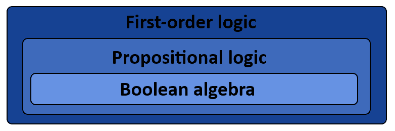
A more formal way to express this idea is to say that the laws of Boolean algebra, which we’ll see shortly, are valid both in propositional and in first-order logic.

3. Terms and Operations

3.1. Boolean Terms

Boolean terms are terms in a Boolean algebraic formula. In contrast with the definition of terms we used in propositional and first-order logic, Boolean terms are simply variables that can assume one and only one of the two values in a binary field. There aren’t any other conditions on them, such as being related to factual knowledge about the world, as was the case for propositional logic; or pertaining to relationships, as was the case for first-order logic.

We can indicate Boolean variables with italic letters of the Latin alphabet, such as $p$ , $q$ , $x$ , and $y$ . Boolean algebra and its laws are built to be valid regardless of the specific values assigned to the variables; therefore, as per the practice of the literature on the subject, we here provide truth tables as a method to prove theorems.

A truth table is simply a table that shows all possible combinations of values for a finite set of Boolean variables. If a set $S = \{s_1, s_2, ..., s_n\}$ contains $|S| = n$ Boolean variables, then the truth table for operations on that set contains $2^n$ rows corresponding to as many different combinations of values for the variables in $S$ :

This table can be interpreted in natural language by reading it row by row. If we start from the first row, we can say: “ $p$ and $q$ are both false”. The second row reads instead “ $p$ is false and $q$ is true”, and we can similarly continue for all others. We can say that two expressions indicated in columns of a truth table are equivalent if all of their values correspond perfectly.

3.2. Basic Boolean Operations

Three basic operations are defined in Boolean algebra, to which correspond as many logical operators. These operators are:

A unary operator $\neg p$ , not p
A binary operator $p\wedge q$ , p and q
And another binary operator $p\vee q$ , p or q

These operators hold the truth values that are enumerated below:

We can read this table in the same way in which we read the previous one. The first row can be read, for example, as “if $p$ and $q$ are both false, then $\text{not } p$ is true, $p \text{ and } q$ is false, and $p \text{ or } q$ is false”. We can, in a similar manner, read all other rows and thus complete the mapping of each operation to its inputs and output.

These operations are called “basic” because all other operations on any number of variables can be reduced to an ordered succession of not, and, and or operations. This is done by repeatedly applying the basic laws to expressions, as we’ll see in the section dedicated to the solution of practical exercises.

3.3. Secondary Operations

We can also define other Boolean operations that we call secondary because of their reducibility to a sequence of basic operations. The most common among these are:

The material conditional $p\to q$ , if p then q
The correspondence or equivalence $p\equiv q$ , p is equivalent to q, or also p if and only if q
The exclusive or operator $p\oplus q$ , p xor q, or also either p or q

These operators are called secondary because they can be reformulated in terms of basic operations:

$p\to q = \neg p\vee q$
$p\equiv q = (p\wedge q)\vee(\neg p\wedge\neg q)$
$p\oplus q = (p\vee q)\wedge(\neg p\vee\neg q)$

The equivalence operator is also sometimes called double conditional and is indicated with a double arrow, facing both variables: $p \leftrightarrow q$ . This notation is particularly used in certain contexts, such as theorem proving, to indicate the interchangeability between a hypothesis and a thesis in a demonstration, but is otherwise of no consequence for our scopes.

The table below shows the demonstration in terms of truth tables of the correspondence between basic and secondary operations:

We can easily test the equivalence between the formulas with secondary operators and those rewritten by using basic operators only. This is done by comparing the respective columns in the tables above, and noticing how they are equivalent regardless of the values assumed by $p$ and $q$ .

4. Basic Laws in Boolean Algebra

4.1. Identity, Annihilator, Idempotence, and Double Negation

The laws in Boolean algebra can be expressed as two series of Boolean terms, comprising of variables, constants, and Boolean operators, and resulting in a valid identity between them. In this sense, if the first term is, for example, the expression $p \wedge q$ and the second term is $q \wedge p$ , the identity $p \wedge q = q \wedge p$ is a law if it’s valid for any values of its variables.

The first class of laws comprises of those that take one single variable as an input, together with constants if necessary. These laws are the identities, the annihilations, and the idempotence with regards to the binary operators.

The first two of these laws comprise of the identities for the two operators $\wedge$ and $\vee$ . The two constants of Boolean algebra, 1 and 0, are the identity elements for, respectively, $\wedge$ and $\vee$ :

The second pair of laws concerns the so-called annihilators. An annihilator is a constant that, when used as input to a binary operator together with a variable, nullifies the contribution that that variable has on the output of the operation. The constants 0 and 1 are, respectively, the annihilator of $\wedge$ and $\vee$ :

The third pair of laws that concern exclusively one variable is the one called idempotence. Any variable $p$ is considered to be idempotent with itself with regards to the operators $\wedge$ and $\vee$ . This is because if that variable is used twice, and if it provides both inputs to the binary operators, then the output of the operator corresponds to the value of that variable:

One last law concerning an individual variable is the so-called law of double negation. This law states that the double application of the negation operator to a single variable corresponds to that variable:

$\neg(\neg p) = p$

4.2. Commutativity and Absorption

The second class of laws concerns the usage of two distinct variables and their relationships. The first group of these is the commutative law of $\wedge$ and $\vee$ . This law states that the output of a basic operator is indifferent from the order in which the two variables are input to it:

The second pair of laws involving two variables concerns the so-called property of absorption of $\wedge$ against $\vee$ , and of $\vee$ against $\wedge$ . This property states that, if any binary operation is performed between two distinct variables, and if the output of this operation is input to the binary operator that wasn’t used, then the first binary operation performed has no influence on the overall outcome of the formula.

In formal notation, the law states that:

$p \wedge (p \vee q) = p$
$p \vee (p \wedge q) = p$

This is the tabular representation of these laws:

4.3. Associativity and Distributivity

The third class comprises the laws that operate on three variables. These laws are the associativity and distributivity properties of the $\wedge$ and $\vee$ operators.

The associativity laws of $\wedge$ and $\vee$ state that a succession of operations involving exclusively one of these operators can be computed in any order, and with the same result:

$(p\wedge q) \wedge r = p\wedge (q\wedge r)$
$(p\vee q) \vee r = p\vee (q\vee r)$

And this is the tabular representation of these laws. Notice how the insertion of a third element forces us to increase the number of rows from $2^2 = 4$ to $2^3 = 8$ :

The last pair of laws concerns the distributive property of $\wedge$ with respect to $\vee$ , and of $\vee$ with respect to $\wedge$ . These laws state that, if a binary operation has as input the output of the other binary operation, then the former can be computed over each of the inputs of the latter without any difference in the overall result. In formal notation, the distributive law corresponds to:

$p\wedge (q\vee r) = (p\wedge q)\vee (p\wedge r)$
$p\vee (q\wedge r) = (p\vee q)\wedge (p\vee r)$

And this is the tabular representation of the distributive laws:

4.4. De Morgan’s Laws

One last set of laws concerns the so-called rules for inference. The rules for inference in a formal system allow the conduct of inferential reasoning over well-formed formulas. In Boolean algebra, the rules for inferential reasoning take the name of De Morgan’s laws.

These laws state that for each basic binary operator, the negation of that operator corresponds to the output of the negation of the inputs to the other operator. In formal terms, they state that:

$\neg (p \wedge q) = \neg p \vee \neg q$
$\neg (p \vee q) = \neg p \wedge \neg q$

We’re going to see how to apply them in an exercise in the next section.

5. Using the Laws of Boolean Algebra

5.1. When Do We Use These Laws

The laws of Boolean algebra allow the simplification of very complex formulas into more manageable expressions. This is particularly important for contexts such as information retrieval where the optimization of the search query may lead to a significant reduction of the time taken to retrieve a target document. This simplification is done by applying the laws of Boolean algebra, such as De Morgan’s laws on otherwise too-complex Boolean expressions.

Another typical application of these laws in programming concerns the simplification of nested if statements, which can be done with the usage of specialized rule engines that simplify the nested statements into shorter forms. One last use case for Boolean laws relates to the simplification of logic circuits, which has recently become mandated by the need to simplify quantum circuits.

In all these cases, the rules that we apply correspond perfectly to the laws that we studied above. In this sense, we can say that Boolean algebra is complete under the laws defined above.

5.2. Exercises With Boolean Laws: Distributive Law

We can now see how to use the Boolean laws to simplify two complex Boolean formulas into more manageable expressions. This section and the next can be read as a guided exercise to the application of Boolean laws.

We can start with this expression:

$F: (\neg p \wedge q) \vee (p \wedge q)$

This expression contains two variables, $p$ and $q$ , and a total of four explicit operators, one unary and both types of binary. The first approach that we can try consists in the application of the distributive law. We know in fact that expressions of the form $(r \wedge s) \vee (r \wedge t)$ are equivalent to $r \vee (s \wedge t)$ .

Because of the distributive law of $\wedge$ over $\vee$ , we can then rewrite the formula first by inverting the order of the terms between brackets, which is possible due to the commutative law:

$F: (q \wedge \neg p) \vee (q \wedge p)$

Then we can extract $q$ , by using the distributive law:

$F: q \vee (\neg p \wedge p)$

Because $(\neg p \wedge p) = 0$ , we can also rewrite the formula as:

$F: q \vee 0$

Finally, because 0 is the identity element of $\vee$ , we can rewrite $F$ by applying the identity law simply as:

$F\prime: q$

This argument demonstrates the equivalence of the expressions $F: (\neg p \wedge q) \vee (p \wedge q)$ and $F\prime: q$ , allowing us to simplify the first to the second.

5.3. Exercises With Boolean Laws: De Morgan

We can now see a guided exercise in the application of De Morgan’s laws. Let’s consider this formula:

$F: \neg (p \wedge \neg (q \vee r))$

Notice how the term $\neg (q \vee r)$ corresponds to the second law of De Morgan that we defined above. We can then replace the term $\neg (q \vee r)$ with $(\neg q \wedge \neg r)$ :

$F: \neg (p \wedge (\neg q \wedge \neg r))$

The whole formula now resembles the first law of De Morgan, which means that we can replace it with its equivalent:

$F: \neg p \vee \neg (\neg q \wedge \neg r)$

One final application of De Morgan to the expression within brackets then gives us $F\prime$ :

$F\prime: \neg p \vee q \vee r$

$F\prime$ is, understandably, a lot more manageable than the original expression, while simultaneously being equivalent to it:

$F = F\prime \to \neg (p \wedge \neg (q \vee r)) = \neg p \vee q \vee r$

Notice lastly how the methods we have used can be replicated algorithmically. Two such algorithmic methods, K-map, and the Quine-McCluskey algorithm are commonly used in computer science. They’re based upon the application of rules for Boolean algebra and perform automatic simplification of Boolean functions, allowing, in turn, the extraction of simple formulas out of complex expressions.

6. Conclusions

In this article, we studied the basic laws of Boolean algebra and showed how to apply them for the simplification of Boolean expressions.

First, we discussed the Boolean operators in terms of truth tables. We also observed how secondary operators can always be expressed in terms of the basic ones.

We then studied the basic laws in their formal notation and also their associated truth tables. In doing so, we learned how to prove that these laws are valid for all values of their variables.

Lastly, we studied how to apply the basic laws of Boolean algebra for the simplification of some complex Boolean expressions. In particular, we saw how to apply the distributive law and De Morgan’s laws for the solution of training exercises.

Full Archive

About Baeldung

Core Concepts

Operating Systems

Artificial Intelligence

Graph Theory

Latex