k-Nearest Neighbors and High Dimensional Data | Baeldung on Computer Science

1. Introduction

In this tutorial, we’ll learn about the k-Nearest Neighbors algorithm. It is a fundamental machine learning model. We can apply for both classification and regression tasks. Yet, applying it to classification tasks is more common.

We’ll explore how to choose the $k$ value and distance metric to increase accuracy. Then, we’ll analyze how the algorithm behaves on high-dimensional data sets. We’ll conclude by mentioning potential cures for issues related to high dimensionality.

2. k-Nearest Neighbors

The k-Nearest Neighbors (k-NN) algorithm assumes similar items are near each other. So, we decide on a data point by examining its nearest neighbors.

To predict the outcome of a new observation, we evaluate the $k$ nearest past observations. We base the prediction on these neighboring observations’ values. We can directly take an average or use a weighted average.

The k-NN algorithm has several advantages:

The main idea is simple and easy to implement
It’s instance-based and doesn’t require an additional training phase
The algorithm is suitable for both classification and regression tasks
We can add new observations to the dataset at any time easily
The output is easy to understand and interpret
We have only one hyper-parameter to tune ( $k$ )

On the other side, there are some disadvantages:

The algorithm depends on past observations
It’s very sensitive to noisy data, outliers, and missing values
It requires data preprocessing such as feature scaling, as it needs homogeneous features
It’s hard to work with categorical features
Costly to calculate distance on large datasets
Costly to calculate distance on high-dimensional data

2.1. Choosing the $k$ Value

It is a common practice to choose $\boldsymbol{k}$ as an odd number to eliminate possible ties. Even $k$ values can lead to equal numbers of votes in binary classification.

The choice of hyper-parameter $\boldsymbol{k}$ changes the outcome of the algorithm. Consider a setting where we have observations from two classes, blue and red. Let’s assume 2 of the 3-nearest neighbors are red, but three of the 5-nearest neighbors are blue:

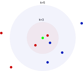
Here, choosing different $k$ values leads to different classification outcomes. So, deciding on the $k$ value is an important step when employing the k-NN algorithm.

Resultingly, the choice of $k$ affects the shape of the decision boundary:

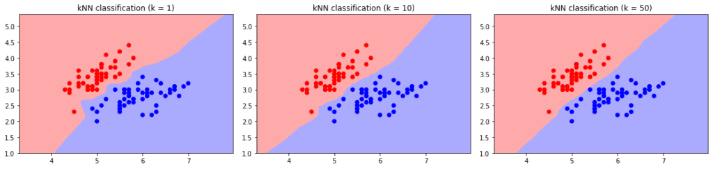
Choosing a large $\boldsymbol{k}$ value leads to high bias by classifying everything as the more probable class. As a result, we have a smooth decision boundary between the classes, with less emphasis on individual points.

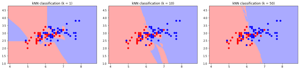
Conversely, small $\boldsymbol{k}$ values cause high variance and an unstable output. Minor changes in the training set cause large changes in classification boundaries. The effect is more visible on intersecting classes:

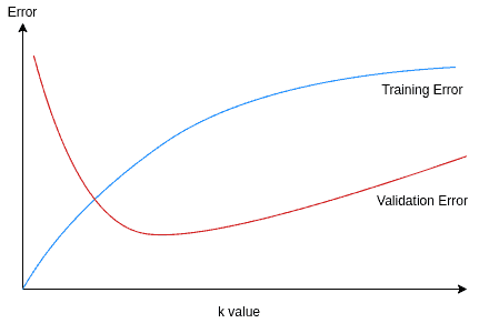
Hence, we need to select the $k$ value based on test and validation sets by observing the outputs. The training and validation errors give a good hint on the behavior of the k-NN classifier.

The training error is minimal (0) for $k$ =1. As $k$ grows, the training error grows as expected. On the other hand, the validation error is high for too small and too large $k$ values. A good choice for the $\boldsymbol{k}$ value is where we have the minimal validation error:

2.2. Distance Functions

The metric used for the distance calculation is not a hyper-parameter for the k-NN algorithm. Still, the distance metric selection changes the outcome and affects the success of the model.

Euclidean distance is the most popular distance metric to calculate distances between data points. However, we need to choose a distance metric depending on the size and dimensions of the dataset at hand.

Let’s explore some well known and commonly used metrics. Minkowski distance is a generalized metric to measure the distance between two points x and y in n dimensional space:

$d\left( x,y\right) = \sqrt[p] {\sum _{i=1}^{n} \left| x_{i}-y_{i}\right|^p }$

Manhattan distance (city-block or L1 distance) is a special case of Minkowski, where we set p=1:

$d\left( x,y\right) = {\sum _{i=1}^{n} \left| x_{i}-y_{i}\right| }$

In other words, the distance between x and y is the sum of absolute differences between their Cartesian coordinates.

Euclidean Distance is another special case of the Minkowski distance, where p=2:

$d\left( x,y\right) = \sqrt {\sum _{i=1}^{n} \left( x_{i}-y_{i}\right)^2 }$

It represents the distance between the points x and y in Euclidean space.

Chebyshev distance is when we have $p \to \infty$ :

$d\left( x,y\right) = max \left( \left| x_{i}-y_{i}\right| \right)$

We can use all variations of the Minkowski difference on real-valued vector spaces. Increasing the $p$ value changes the distance, hence, the decision boundary:

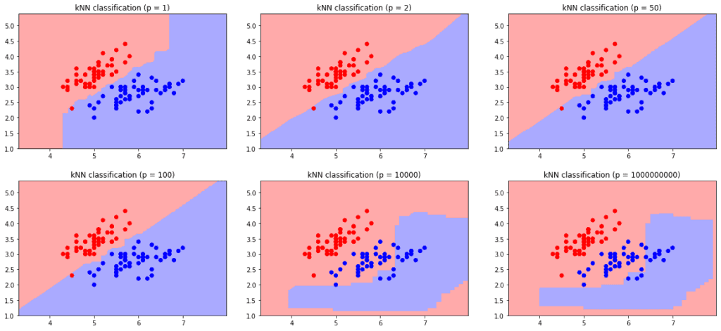
With high-dimensional data sets, using a small $\boldsymbol{p}$ value is more favorable. Because calculating the distance is faster with smaller $p$ values.. Hence, the Manhattan distance is the best option for very high-dimensional datasets.

Hamming distance is a distance measure that we can use for integer-valued vector spaces besides real-valued vectors. It’s usually utilized for comparing strings of equal length by measuring the distance between non-equal characters.

$d\left( x,y\right) = \sum _{i=1}^{k} \left| x_{i}-y_{i}\right|$

Jaccard distance is a measure suitable to find the distance between boolean-valued vectors. It calculates the overlapping features over the entire sample set.

The cosine similarity measure is not a metric, as it doesn’t hold the triangle equality. Yet, it is adopted to classify vector objects such as documents and gene sequences. It measures the frequency of a particular instance in a feature.

3. High Dimensionality

k-NN algorithm’s performance gets worse as the number of features increases. Hence, it’s affected by the curse of dimensionality. Because, in high-dimensional spaces, the k-NN algorithm faces two difficulties:

It becomes computationally more expensive to compute distance and find the nearest neighbors in high-dimensional space
Our assumption of similar points being situated closely breaks

As the number of features increases, the distance between data points becomes less distinctive. Moreover, the total area we need to cover to find $k$ neighbors increase.

Let’s consider a simple setting where our dataset has $f$ number of features, and each feature has a value in the range [0, 1]. We fix $k$ to 10 and $n$ (number of observations) to 1000. Let’s further assume that each feature’s values are uniformly distributed.

In this setting, let’s find out the length of a side of a cube containing $k$ =10 data points.

For example, if $f$ =2, a square of 0.1 $\times$ 0.1 covers 1/100 of the total area, covering 10 data points in total.

If we increment f to $f$ =3, to cover 1/100 of the volume, we need a cube with a side’s length=0.63.

As we keep incrementing $f$ , a side’s length grows exponentially. We can formulate the side’s length $s$ to be:

$s = (k/n)^{1/f}$

We see that with $f$ =100 features, $s$ =0.955. Iterating in a similar manner, $f$ =1000 leads to $s$ =0.995.

As a result, the initial assumption of similar observations being close fails. We can’t say similar observations are clustered closer together in a high-dimensional dataset as the distance between all data points becomes smaller and smaller.

Still, there are ways to represent a dataset in lower dimensions without losing the fundamental structure. Let’s have a look at potential cures:

3.1. Data Reduction

We call representing high-dimensional data in low-dimensional space with keeping the original properties dimension reduction.

We can use a feature selection technique to eliminate more redundant features from the dataset. This method ensures that we only keep the most relevant features.

Alternatively, we can use feature extraction to map the data into a low-dimensional space. The new feature set is not necessarily a subset of the original components. Typically, the new features are generated by combining the existing ones. For example, principal component analysis (PCA) applies linear mapping to maximize information over a minimal number of features.

PCA and kernel methods are especially beneficial when the true dimensionality of the dataset is lower than the actual representation. For example, we can represent the points on a 2-dimensional plane in 3D space with 2 features after a mapping.

Another data reduction technique is to represent data in smaller forms with fewer observations. Numerosity reduction algorithms help with k-NN performance as the number of calculations decreases.

3.2. Use of an Approximate k-NN

In some cases, finding an approximate solution is acceptable. If searching for the exact solution becomes too costly, we can adopt an approximation algorithm without guaranteeing the exact result. High-dimensional similarity search techniques give a fast approximation for k-NN in a high-dimensional setting.

Locality sensitive hashing (LSH) algorithm hashes similar items into high-probability buckets. We expect similar items to end up in the same buckets at the end, as the name suggests.

The use of hash tables is easy and efficient, both for querying and data generation. This way, the LSH method is used to find approximate nearest neighbors fast.

Random projections allow us to transform m points from a high-dimensional space into only $\mathcal{O}(log m/\epsilon^2)$ dimensions by changing the distance between any two points by a factor of ( $1\pm \epsilon$ ). Therefore, the mapping preserves the Euclidean distances. So, running the k-NN algorithm generates the same result at a much lower cost.

Random projection forests (rpForests) perform fast approximate clustering. They approximate the nearest neighbors quickly and efficiently.

4. Conclusion

In this article, we’ve explored the k-NN algorithm. We’ve analyzed how a change in a hyper-parameter affects the outcome and how to tune its hyper-parameters.

Then, we’ve examined the k-NN algorithm’s behavior on high-dimensional data sets. Last, we’ve discussed how we can overcome performance issues by the use of approximation algorithms.

Full Archive

About Baeldung

Core Concepts

Operating Systems

Artificial Intelligence

Graph Theory

Latex