Fast Gaussian Blur Implementation in Java

1. Introduction

Gaussian blur is a widely used image processing technique for reducing image noise and detail. However, achieving accurate Gaussian blur can be computationally expensive, especially for high-resolution images with large blur radii.

In this tutorial, we’ll explore a faster, more computationally efficient solution for implementing Gaussian blur in Java.

2. Problem Overview

We implement a standard Gaussian blur on a grayscale image by convolving it with a 2D Gaussian kernel. Here, for each pixel in an image, the algorithm first examines a surrounding grid of pixels (the kernel). Then, it multiplies each pixel’s intensity by a specific weight. Finally, it sums them up.

For an image with n pixels and a blur radius of r, our kernel size is (2r + 1)  x  (2r + 1). Thus, the standard 2D convolution algorithm has a time complexity of O(n.r²). As the blur radius r grows, the performance degrades quadratically. Thus, it is not optimal for real-time processing over large images.

3. The Fast Approximation Algorithm

Our fast approximations make two key enhancements to the standard Gaussian 2D blur method.

3.1. Separable Filters

A 2D Gaussian kernel can be seen and used as two 1D Gaussian vectors. In other words, we can separate them as horizontal and vertical vectors. So, instead of applying a 2D matrix to every pixel of the image, we can achieve the same result by applying a horizontal 1D blur across all rows, followed by a vertical 1D blur down all columns.

This simple separation reduces our average-case time complexity from O(n.r²) to O(n.r).

3.2. Repeated Box Blurs

We repeat a specific blur operation (box blur) to achieve the desired effect.

We define box blur as the simplest form of blurring, assigning equal weight to every pixel within the blur radius. Then, we make use of the Central Limit Theorem to approximate a valid and matching Gaussian distribution. According to the Central Limit Theorem, applying a simple Box Blur multiple times closely approximates an accurate Gaussian distribution. We run five consecutive passes of a box blur to get a visually indistinguishable result from a strict Gaussian blur with a fraction of the computational overhead.

Furthermore, we make all weights in a Box Blur equal, so we don’t need to re-sum the entire radius for every pixel. This gives us the freedom to use a sliding window or a moving average. As the window shifts to the right by one pixel, we subtract the leaving pixel and add the entering pixel. This drops our average time complexity to O(n), making the performance entirely independent of the blur radius r!

4. Solution

Let’s move to the solution.

4.1. The Sliding Window Box Blur

First, we define a function, horizontalBoxBlur(), that performs a 1D horizontal blur using the sliding-window technique.

Here, we process the image row by row. We don’t recalculate the pixel sum at every position. Instead, we initialize windowSum for the very first pixel in a row. As it moves left to right, it subtracts the value of the pixel beyond the trailing edge of the radius and adds the value of the pixel at the leading edge.

Lastly, we clamp edges to ensure that if the radius extends beyond the image boundaries, our logic duplicates the edge pixels rather than throwing an ArrayIndexOutOfBoundsException.

private static void horizontalBoxBlur(int[] source, int[] target, int width, int height, int radius) {
    double scale = 1.0 / (radius * 2 + 1);
    for (int y = 0; y < height; y++) {
        int windowSum = 0;
        int offset = y * width;        
        for (int x = -radius; x <= radius; x++) {
            int safeX = Math.min(Math.max(x, 0), width - 1);
            windowSum += source[offset + safeX];
        }        
        for (int x = 0; x < width; x++) {
            target[offset + x] = (int) Math.round(windowSum * scale);
            int leftX = Math.max(x - radius, 0);
            int rightX = Math.min(x + radius + 1, width - 1);
            windowSum -= source[offset + leftX];
            windowSum += source[offset + rightX];
        }
    }
}

The verticalBoxBlur() is identical in logic, but here we traverse columns rather than rows (top to bottom):

private static void verticalBoxBlur(int[] source, int[] target, int width, int height, int radius) {
    double scale = 1.0 / (radius * 2 + 1);
    for (int x = 0; x < width; x++) {
        int windowSum = 0;
        for (int y = -radius; y <= radius; y++) {
            int safeY = Math.min(Math.max(y, 0), height - 1);
            windowSum += source[safeY * width + x];
        }
        for (int y = 0; y < height; y++) {
            target[y * width + x] = (int) Math.round(windowSum * scale);
            int topY = Math.max(y - radius, 0);
            int bottomY = Math.min(y + radius + 1, height - 1);
            windowSum -= source[topY * width + x];
            windowSum += source[bottomY * width + x];
        }
    }
}

4.2.  Integration

This is our orchestrator.

Leveraging the Central Limit Theorem, we apply a horizontal and vertical box blur three times (configurable). This smooths out peaky regions, thus creating a near-perfect approximation of a true Gaussian bell curve. It uses a temp array (temp) to safely ping-pong the data between passes without corrupting the source:

public static int[] applyFastGaussianBlur(int[] source, int numPasses, int width, int height, int radius) {
    int[] target = new int[source.length];
    int[] temp = new int[source.length];
    System.arraycopy(source, 0, target, 0, source.length);
    for (int i = 0; i < numPasses; i++) {
        horizontalBoxBlur(target, temp, width, height, radius);
        verticalBoxBlur(temp, target, width, height, radius);
    }
    return target;
}

5. Test

5.1. Test Using Impulse Image

First, let’s test this method using an impulse image (artificial images with a single black pixel). Our main objective is to verify if  our algorithm handles edges correctly and applies a smoothing effect:

void givenSharpImage_whenAppliedBlur_thenCenterIsSmoothed() {
    int width = 5;
    int height = 5;
    int numPasses = 5;
    int[] image = new int[width * height];
    image[12] = 255; 
    int[] blurredImage = FastGaussianBlur.applyFastGaussianBlur(image, numPasses, width, height, 1);
    assertTrue(blurredImage[12] < 255);
    assertTrue(blurredImage[12] > 0);
    assertTrue(blurredImage[11] > 0); // Left neighbor
    assertTrue(blurredImage[13] > 0); // Right neighbor
}

We begin by creating a 5×5 image (25 pixels) and set all pixels to 0, making them pure black. Then we set the exact center pixel (index 12) to 255, making it pure white. This sharp point is our impulse or peak. Then we apply the fast blur algorithm with a radius of 1.

Our main claim is that blur, when applied correctly, spreads the brightness of the central pixel outwards into the surrounding black pixels. Further, assertTrue(blurredImage[12] < 255) confirms the center pixel has dimmed because it shared its brightness, and assertTrue(blurredImage[11] > 0) and assertTrue(blurredImage[13] > 0) confirm that the immediate left and right neighbors (both black) have absorbed that dispersed brightness.

5.2. Test Using Real Image

We take an open-source image and blur it using our algorithm. Here is the sample image:

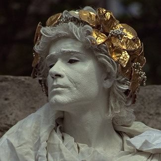
Please check the blurred version:

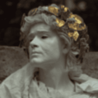
We used a single channel of integer values for our impulse image (grayscale) test case. For this case, we use real images. Each real image is packed with 32-bit ARGB (Alpha, Red, Green, Blue) data. So, here we extract the ARGB channels, then blur each of the RGB channels independently, and finally pack them back together:

public static BufferedImage blurRealImage(@Nonnull BufferedImage image, int radius, int numPasses) {
    int width = image.getWidth();
    int height = image.getHeight();
    int[] pixels = image.getRGB(0, 0, width, height, null, 0, width);

    int[] a = new int[pixels.length];
    int[] r = new int[pixels.length];
    int[] g = new int[pixels.length];
    int[] b = new int[pixels.length];

    for (int i = 0; i < pixels.length; i++) {
        a[i] = (pixels[i] >> 24) & 0xff;
        r[i] = (pixels[i] >> 16) & 0xff;
        g[i] = (pixels[i] >> 8) & 0xff;
        b[i] = pixels[i] & 0xff;
    }

    r = FastGaussianBlur.applyFastGaussianBlur(r, width, height, radius, numPasses);
    g = FastGaussianBlur.applyFastGaussianBlur(g, width, height, radius, numPasses);
    b = FastGaussianBlur.applyFastGaussianBlur(b, width, height, radius, numPasses);

    int[] resultPixels = new int[pixels.length];
    for (int i = 0; i < pixels.length; i++) {
        resultPixels[i] = (a[i] << 24) | (r[i] << 16) | (g[i] << 8) | b[i];
    }

    BufferedImage result = new BufferedImage(width, height, BufferedImage.TYPE_INT_ARGB);
    result.setRGB(0, 0, width, height, resultPixels, 0, width);
    return result;
}

6. Conclusion

In this article, we learned a faster Gaussian blur method in Java. We made two key enhancements to the standard Gaussian blur implementation to achieve linear time complexity. First, we decomposed a 2D convolution matrix into separable 1D arrays, and second, we used a moving-average sliding window across three box-blur passes. Thus, our solution works in a constant processing time that is independent of the blur radius.

As always, the complete code examples are available over on GitHub.