Yes, we're now running our only Summer Sale. All Courses are 30% off until 20th July, 2026:
Gaussian Mixture Models
Last updated: February 28, 2025

Learn through the super-clean Baeldung Pro experience:
>> Membership and Baeldung Pro.
No ads, dark-mode and 6 months free of IntelliJ Idea Ultimate to start with.
1. Introduction
Machine learning and data science unquestionably use Gaussian Mixture Models as a powerful statistical tool. Probabilistic models use Gaussian Mixture Models to estimate density and cluster data. Moreover, it is important to realize that Gaussian Mixture Models are extremely beneficial when dealing with data that appears to combine numerous Gaussian distributions.
In this tutorial, we’ll learn about Gaussian Mixture Models.
2. Gaussian Mixture Models Overview
Gaussian Mixture Model blends multiple Gaussian distributions. In other words, the Gaussian distribution parameters calculate each cluster’s mean, variance and weight. Hence, we can determine the probabilities of each point belonging to each cluster after learning the parameters of each point.
3. Steps
A Gaussian Mixture Model is the weighted sum of several Gaussian distributions. Accordingly, the model attempts to assign data points to the appropriate cluster based on their likelihood of belonging to each component. Namely, each Gaussian distribution in the mixture corresponds to a data cluster. Here’s a step-by-step description of Gaussian Mixture Models.
3.1. Model Representation
Gaussian components are linearly combined to form a Gaussian Mixture Model. In general, they use the mean, covariance matrices, and weights of each component as indicators. Given that the probability density function of a Gaussian Mixture Model is the sum of the probability density functions of its Gaussian components, weighted by the probabilities assigned to each.
Notation:
 : The Gaussian Mixture Model’s number of Gaussian components or clusters
 : Number of data points in the dataset
 : Dimensionality (the number of characteristics)
Gaussian Mixture Model Parameters:
Means (μ): These represent the locations of the centers of each Gaussian component. Each component has a mean vector of D length.
Covariance Matrices (Σ): Covariance matrices define each Gaussian component’s shape and distribution A  size covariance matrix is present for each component.
Weights (π): The probability of selecting each component is represented by weights. 0 ≤ π_i ≤ 1 and Σ(π_i) = 1 are satisfied. Please note that π_i represents the weight of the i-th component.
3.2. Model Training
To train a Gaussian Mixture Model, the parameters (means, covariance, and weights) must be established using the available dataset.
When training Gaussian Mixture Models, the Expectation-Maximization technique is frequently employed. In essence, until convergence, the Expectation ( ) and Maximization (
 ) steps are alternated.
3.3. Expectation-Maximization
Let’s keep going through stages E and M. Based on the current model parameters, the expectation () stage of the procedure calculates the posterior probabilities of each data point belonging to each Gaussian component. The algorithm modifies the model’s parameters (means, covariance matrices, and weights) in the maximization () phase using the information from the weighted data points from the E-step.
3.4. Clustering and Density Estimation
After training, data points can be clustered using the Gaussian Mixture Model. For each data point, the cluster with the highest posterior probability is assigned. Therefore, Gaussian Mixture Models for density estimation can be used to estimate the probability density at every point in the feature space.
4. Implementation of Gaussian Mixture Models
After understanding the concept and steps of the Gaussian Mixture Models, let’s look at the flowchart of the Gaussian Mixture Models. For instance, this is the flowchart for the Gaussian Mixture Model:
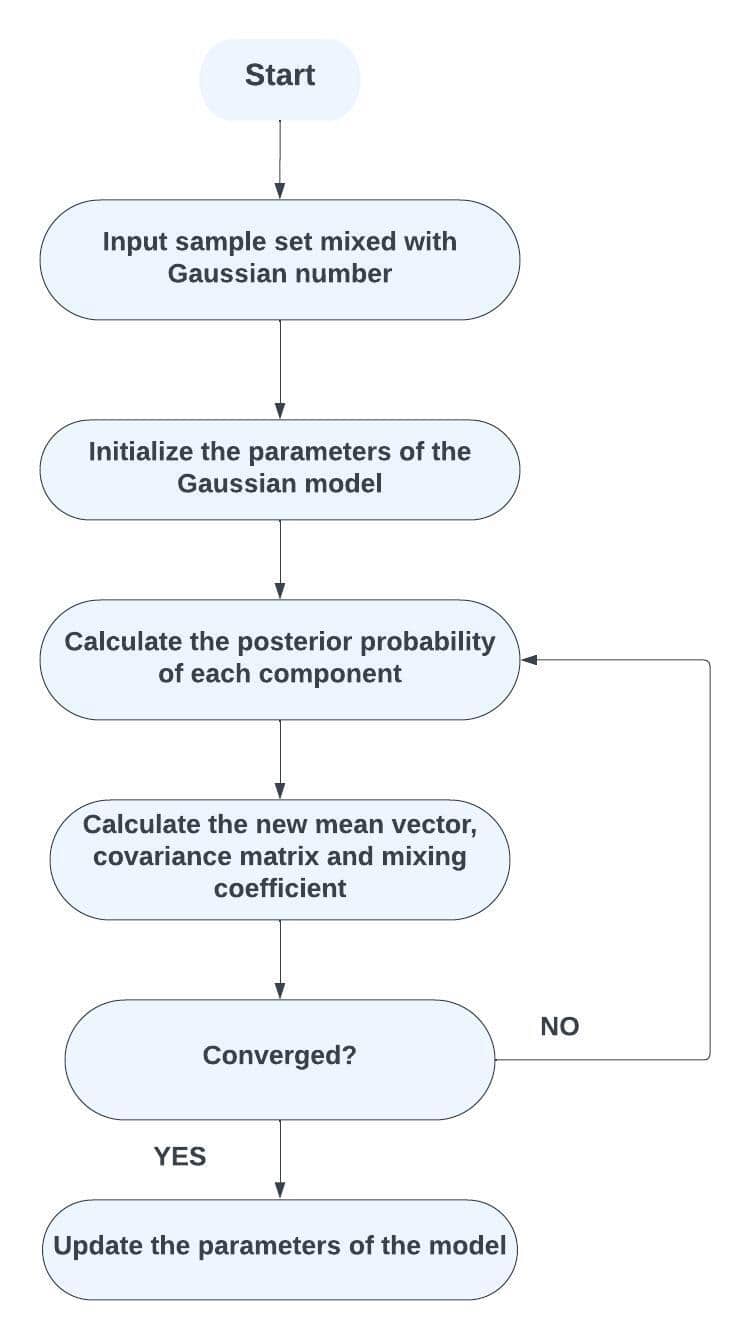
Specifically, the implementation of the Gaussian Mixture Model in Python can be found here.
5. Use Cases of Gaussian Mixture Models
The applications of Gaussian Mixture Models include anomaly detection, image segmentation, and speech recognition.
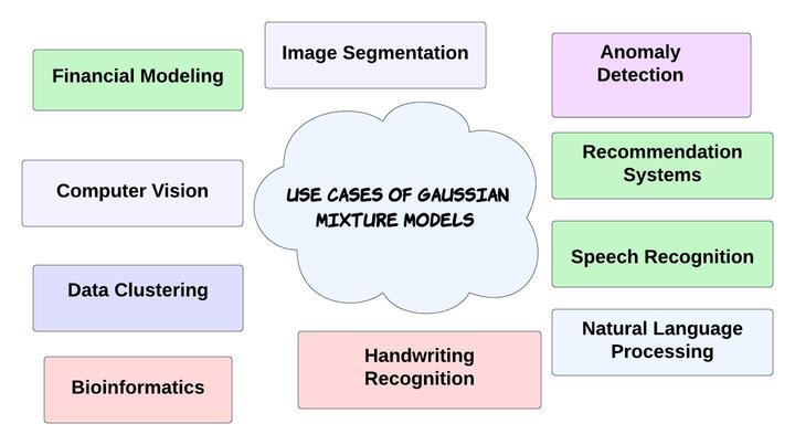
Gaussian Mixture Models are flexible in managing complex data distributions. Consequently, a wide range of industries use these models.
GMMs can segment images by grouping pixels into various regions based on their colour or texture characteristics. Because each region corresponds to a Gaussian component-represented cluster.
We can use GMMs to discover anomalies in datasets. For instance, the model can detect deviations from normal behaviour by assigning low probabilities to anomalies. Automatic speech recognition systems employ GMMs to simulate the acoustic features of phonemes. For this purpose, they aid in the mapping of auditory properties to phonetic units. Finally, this allows speech recognition based on these acoustic models.
We can also use GMMs to simulate a variety of handwriting styles for each character or word in handwriting recognition tasks, allowing for more robust recognition. GMMs can help in customer segmentation and market research to group customers with comparable behaviours or preferences.
Data clustering is the process of finding natural groups or clusters in the data using GMMs. Furthermore, a Gaussian component represents each cluster, and probabilities sort data points into clusters.
Computer vision tasks, including object detection, tracking, and background removal from video sequences, all make use of GMMs.
Bioinformatics uses GMMs to model gene expression data and detect patterns or clusters of gene expression profiles. Recommendation systems can use GMMs to model user preferences and item attributes for individualized recommendations. Medical image analysis employs GMMs for picture segmentation, tissue classification, and spotting aberrant areas in images.
Finance uses GMMs to model changes in asset prices. In addition to helping with option pricing, risk control, and portfolio optimization. Thus, Gaussian Mixture Models can be used to predict underlying price distributions.
6. Advantages and Disadvantages of Gaussian Mixture Models
Machine learning and data analysis applications widely use Gaussian Mixture Models since they have many advantages:
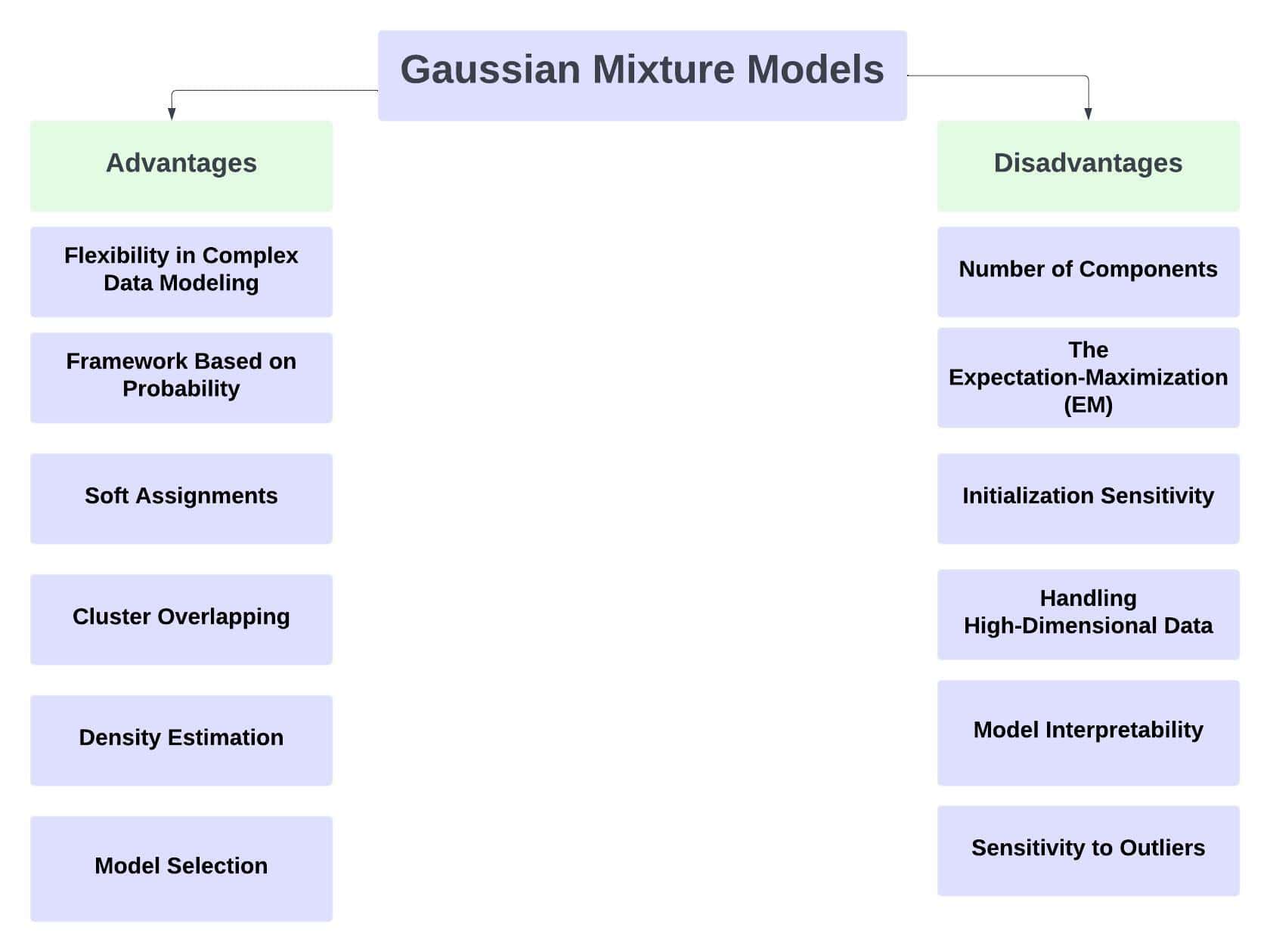
6.1. Advantages of Gaussian Mixture Models
GMMs are good at approximating complex data distributions. For that reason, they are appropriate for datasets with complicated underlying structures. Because they may represent data with various clusters.
They also offer a probabilistic method for modelling data. Furthermore, Gaussian Mixture Models assign probabilities to the data points corresponding to each cluster to enable uncertainty estimation and confidence measures for each assignment.
GMMs offer soft cluster assignments compared to hard clustering methods (like k-means). For instance, when a data point is a member of more than one cluster, it is probabilistically assigned to each cluster. Consequently, this allows greater flexibility.
Since each cluster is represented as a Gaussian distribution with its own covariance matrix, GMMs successfully model data with overlapping clusters. Therefore, this trait is especially helpful when clusters aren’t clearly separated in feature space. GMMs are useful for density estimation applications because they can estimate the data’s underlying probability density function. Accordingly, this can be helpful in situations where understanding the distribution and form of the data is crucial.
Specifically, GMMs are naturally capable of handling missing data. Thus, even if some characteristics are missing, the model can nevertheless estimate the Gaussian parameters using the data that is currently available.
Data points with low probability under the fitted model are probably anomalies or outliers, hence GMMs can be utilized for outlier detection.
GMMs scale well to big datasets and are very simple to implement. Thus, iterative parameter estimation using the Expectation-Maximization algorithm is an effective technique for GMM training.
Interpretable information about the features of each cluster is provided by the model parameters of GMMs, such as cluster means and covariance matrices.
6.2. Disadvantages of Gaussian Mixture Models
Particularly, choosing the right number of Gaussian clusters for a GMM model is one of the main issues. For instance, incorrectly choosing the number of components can cause the data to be over-fitted or under-fitted.
Surprisingly, the initializations of the means, covariance, and weights of the Gaussian components impact GMM training. Because different initializations can produce various outcomes and converge to various local optimum states. Hence, to address this problem, many restarts of the EM algorithm with various initializations are frequently necessary. As a result, this becomes a disadvantage.
Generally, there is an assumption that all sorts of data are produced by a combination of Gaussian distributions. Surprisingly, this is not always true. Accordingly, GMMs might not be the best model if the data have non-Gaussian forms or don’t have a Gaussian distribution.
Most importantly, the “curse of dimensionality” can affect GMMs in high-dimensional domains. The amount of information required to precisely estimate the model parameters grows exponentially as the number of characteristics rises. Moreover, if there is a small amount of data, this may result in overfitting or inaccurate outcomes.
Notably, if one of the Gaussian components has a singular covariance matrix (low-rank), GMMs may experience convergence problems. Particularly, this circumstance may occur when one cluster’s data is located in a lower-dimensional subspace.
Especially, GMMs can function well with moderate-sized datasets. Conversely, if the data size increases significantly, their memory and computing needs may become prohibitive.
Although interpretable parameters like cluster mean and covariance are provided by GMMs, the interpretation may be difficult if the dataset has a high degree of dimensionality and many components.
Specifically, the potential impact that outliers may have on the estimate of Gaussian parameters. Thus, GMMs are susceptible to them.
6.3. Overall
Regardless of their benefits, GMMs also have certain drawbacks. For instance, their sensitivity to parameter initialization and the requirement that the number of Gaussian components be specified. Importantly, inappropriate component selection might result in either overfitting or underfitting. Therefore, to maximize the use of Gaussian Mixture Models in various applications, careful study and model validation are required.
On the other hand, Gaussian Mixture Models continue to be an effective tool in many contexts despite these drawbacks. Undoubtedly, it is essential to consider the individual characteristics of the data and the modelling objectives before selecting GMMs.
7. Conclusion
In this article, we learned about the definition, steps, implementation, use cases, advantages, and disadvantages of Gaussian Mixture Models. Gaussian Mixture Models are a powerful and widely used statistical tool in machine learning and data analysis.