2D Convolution as a Matrix-Matrix Multiplication

1. Introduction

In this tutorial, we’ll show a matrix approach to do 2D convolution.

2. Convolution

Convolution is fundamental in signal processing, computer vision, and machine learning. It applies a filter or kernel to an input image or signal and extracts relevant features.

Typical implementations use a sliding-window operation where the kernel moves across the input image. For each placement of the kernel $K$ on the input image $A$ , we compute the dot product of the kernel and the overlapping image pixels:

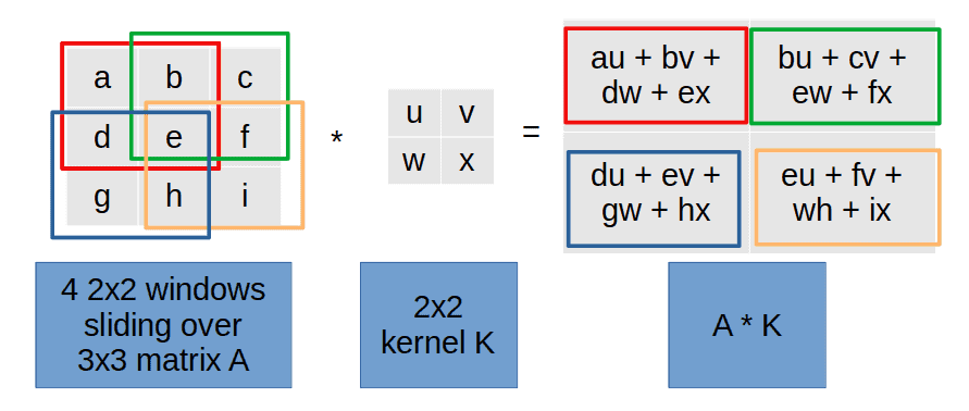
However, the kernel approach can be computationally expensive, especially for large images and kernels. An alternative is to compute convolution as matrix multiplication, which can be a more efficient approach.

3. Matrix Construction of a 2D Convolution

Let $A$ be a matrix of size $n\times n$ and $K$ a $k\times k$ kernel. For convenience, let $t = n - k + 1$ .

To calculate the convolution $A * K$ , we need to calculate the matrix-vector multiplication $Mv^T = v'^T$ where:

$M$ is a $t^2 \times n^2$ block matrix we get from the kernel $K$
$v$ is a row vector with the $n^2$ elements of $A$ concatenated row by row
$v'$ is a row vector of $t^2$ elements which can be reshaped into a $t\times t$ matrix by splitting the row vector into $t$ rows of $t$ elements

3.1. How to Compute the Block Matrix?

It’s a three-step process.

First, we define the $K_i$ matrixes, which represent all the horizontal sliding windows for kernel row $i$ :

$K_i = \begin{bmatrix}0_{0} & K_{i,1} & \hdots & K_{i, k} & 0_{t - 1} \\ 0_{1} & K_{i,1}& \hdots & K_{i, k} & 0_{t - 2} \\ \hdots & \hdots & \hdots & \hdots & \hdots \\ 0_{t-1} & K_{i,1} & \hdots & K_{i, k}& 0_{0}\end{bmatrix}$

with $0_j$ a zero row vector of size $0 \leq j\leq n - k$ and $K_{i,j}$ the $j$ -th element of row $K_i$ , i.e. the element at row $i$ and column $j$ in matrix $K$ . $0_0$ stands for an empty vector.

In the second step, we complete horizontal sliding by constructing a $t \times kn$ matrix $\hat{K}$ . We define $\hat{K}$ as the horizontal concatenation of matrix blocks $K_i$ :

$\hat{K} = (K_1 K_2 \hdots K_k)$

The final step is to represent vertical window sliding. We do that by padding $\hat{K}$ with zero matrices (denoted $0_{u\times v}$ ):

$M = \begin{bmatrix}0_{t\times 0} & \hat{K} & 0_{t\times n(t-1)} \\ 0_{t\times n} & \hat{K} & 0_{t\times n(t-2)} \\ \hdots & \hdots & \hdots \\ 0_{t\times n(t-1)} & \hat{K} & 0_{t\times 0} \end{bmatrix}$

All that is now left to do is compute $Mv$ , where $v=(a_{11}, a_{12}, \ldots, a_{nn})$ is a row-vector form of the input matrix $A$ .

4. Example

Let’s construct the matrix $M$ for a $3\times 3$ matrix $A$ convolved with a $2 \times 2$ kernel $K$ :

$A = \begin{bmatrix}a_{1,1} & a_{1,2} & a_{1,3} \\ a_{2,1} & a_{2,2} & a_{2,3} \\ a_{3,1} & a_{3,2} & a_{3,3}\end{bmatrix}\qquad K = \begin{bmatrix}k_{1,1} & k_{1,2} \\ k_{2,1} & k_{2,2} \end{bmatrix}$

In this example, we have $t = n - k + 1 = 3 - 2 + 1 = 2$ . First, we build the blocks $K_1$ and $K_2$ :

$K_1 = \begin{bmatrix}k_{1,1} & k_{1,2} & 0 \\ 0 & k_{1,1} & k_{1,2}\end{bmatrix}, K_2 = \begin{bmatrix}k_{2,1} & k_{2,2} & 0 \\ 0 & k_{2,1} & k_{2,2}\end{bmatrix},$

and get $\hat{K}$ after concatenation:

$\hat{K} = \begin{bmatrix}k_{1,1} & k_{1,2} & 0 & k_{2,1} & k_{2,2} & 0 \\ 0 & k_{1,1} & k_{1,2} & 0 & k_{2,1} & k_{2,2}\end{bmatrix}$

The final step is to pad the matrix with blocks of zeros:

$\setcounter{MaxMatrixCols}{20} M = \begin{bmatrix}k_{1,1} & k_{1,2} & 0 & k_{2,1} & k_{2,2} & 0 & 0 & 0 & 0 \\ 0 & k_{1,1} & k_{1,2} & 0 & k_{2,1} & k_{2,2} & 0 & 0 & 0 \\ 0 & 0 & 0 & k_{1,1} & k_{1,2} & 0 & k_{2,1} & k_{2,2} & 0 \\ 0 & 0 & 0 & 0 & k_{1,1} & k_{1,2} & 0 & k_{2,1} & k_{2,2}\end{bmatrix}$

The zeros in the $2\times 3$ matrix blocks are highlighted in red, and $M$ is exactly of the size $t^2 \times n^2 = 4\times 9$ .

Now, let’s rewrite $A$ as $v$ :

$\setcounter{MaxMatrixCols}{20} v = \begin{bmatrix}a_{1,1} & a_{1,2} & a_{1,3} & a_{2,1} & a_{2,2} & a_{2,3} & a_{3,1} & a_{3,2} & a_{3,3}\end{bmatrix}$

Finally, we multiply $M$ and $v$ :

$\setcounter{MaxMatrixCols}{20} Mv^T = \begin{bmatrix} a_{1,1}k_{1, 1} + a_{1,2}k_{1, 2} + a_{1,3}\cdot 0 + a_{2,1}k_{2, 1} + a_{2,2}k_{2, 2} + a_{2,3}\cdot 0 + a_{3,1}\cdot 0 + a_{3,2}\cdot 0 + a_{3,3} \cdot 0 \\a_{1,1}\cdot 0 + a_{1,2}k_{1, 1} + a_{1,3}k_{1,2} + a_{2,1}\cdot 0 + a_{2,2}k_{2, 1} + a_{2,3}k_{2,2} + a_{3,1}\cdot 0 + a_{3,2}\cdot 0 + a_{3,3} \cdot 0 \\a_{1,1}\cdot 0 + a_{1,2}\cdot 0 + a_{1,3} \cdot 0 + a_{2,1}k_{1, 1} + a_{2,2}k_{1, 2} + a_{2,3}\cdot 0 + a_{3,1}k_{2, 1} + a_{3,2}k_{2, 2} + a_{2,3}\cdot 0 \\a_{1,1}\cdot 0 + a_{1,2}\cdot 0 + a_{1,3} \cdot 0 + a_{2,1}\cdot 0 + a_{2,2}k_{1, 1} + a_{2,3}k_{1,2} + a_{3,1}\cdot 0 + a_{3,2}k_{2, 1} + a_{3,3}k_{2,2} \end{bmatrix}$

Since $Mv^T=v'^T$ , we obtain the result of the convolution $A * K$ as a $t\times t = 2\times 2$ matrix by simplifying and reshaping $v'$ :

$\begin{bmatrix}a_{1,1}k_{1, 1} + a_{1,2}k_{1, 2} + a_{2,1}k_{2, 1} + a_{2,2}k_{2, 2} & a_{1,2}k_{1, 1} + a_{1,3}k_{1,2} + a_{2,2}k_{2, 1} + a_{2,3}k_{2,2} \\ a_{2,1}k_{1, 1} + a_{2,2}k_{1, 2} + a_{3,1}k_{2, 1} + a_{3,2}k_{2, 2} & a_{2,2}k_{1, 1} + a_{2,3}k_{1,2} + a_{3,2}k_{2, 1} + a_{3,3}k_{2,2} \\\end{bmatrix}$

4.1. Numeric Example

Let’s say $A$ and $K$ are:

$A = \begin{bmatrix}1 & 2 & 3 \\ 4 & 5 & 6 \\ 7 & 8 & 9\end{bmatrix} \qquad K = \begin{bmatrix}10 & 11 \\ 12 & 13\end{bmatrix}$

The corresponding $v$ , $\hat{K}$ , and $M$ are as follows:

$v^T = \begin{bmatrix}1 \\ 2 \\ 3 \\ 4 \\ 5 \\ 6 \\ 7 \\ 8 \\ 9\end{bmatrix} \qquad\hat{K} = \begin{bmatrix}10 & 11 & 0 & 12 & 13 & 0 \\ 0 & 10 & 11 & 0 & 12 & 13\end{bmatrix} \qquad M = \begin{bmatrix}10 & 11 & 0 & 12 & 13 & 0 & 0 & 0 & 0 \\ 0 & 10 & 11 & 0 & 12 & 13 & 0 & 0 & 0 \\ 0 & 0 & 0 & 10 & 11 & 0 & 12 & 13 & 0 \\ 0 & 0 & 0 & 0 & 10 & 11 & 0 & 12 & 13\end{bmatrix}$

The result of the convolution is:

$Mv^T = \begin{bmatrix}1\cdot 10 + 2\cdot 11 + 3\cdot 0 + 4\cdot 12 + 5\cdot 13 + 6\cdot 0 + 0\cdot 7 + 0\cdot 8 + 0\cdot 9 \\1\cdot 0 + 2\cdot 10 + 3\cdot 11 + 4\cdot 0 + 5\cdot 12 + 6\cdot 13 + 0\cdot 7 + 0\cdot 8 + 0\cdot 9 \\0\cdot 1 + 0\cdot 1 + 0\cdot 3 + 4\cdot 10 + 5\cdot 11 + 6\cdot 0 + 7\cdot 12 + 8\cdot 13 + 6\cdot 0 \\0\cdot 1 + 0\cdot 1 + 0\cdot 3 + 4\cdot 0 + 5\cdot 10 + 6\cdot 11 + 7\cdot 0 + 8\cdot 12 + 9\cdot 13 \\ \end{bmatrix} =\begin{bmatrix}145 \\191 \\283 \\329 \\\end{bmatrix}$

We can reshape $Mv^T$ :

$\begin{bmatrix}1\cdot 10 + 2\cdot 11 + 4\cdot 12 + 5\cdot 13 & 2\cdot 10 + 3\cdot 11 + 5\cdot 12 + 6\cdot 13 \\ 4\cdot 10 + 5\cdot 11 + 7\cdot 12 + 8\cdot 13 & 5\cdot 10 + 6\cdot 11 + 8\cdot 12 + 9\cdot 13 \\\end{bmatrix} =\begin{bmatrix}145 & 191 \\283 & 329 \\\end{bmatrix}$

5. Advantages of the Matrix Approach

Matrix multiplication is easier to compute compared to a 2D convolution because it can be efficiently implemented using hardware-accelerated linear algebra libraries, such as BLAS (Basic Linear Algebra Subprograms). These libraries have been optimized for many years to achieve high performance on a variety of hardware platforms.

In addition, the memory access patterns for matrix multiplication are more regular and predictable compared to 2D convolution, which can lead to better cache utilization and fewer memory stalls. This can result in faster execution times and better performance.

6. Conclusion

In this article, we showed how to compute a convolution as a matrix-vector multiplication. The approach can be faster than the usual one with sliding since matrix operations have fast implementations on modern computers.

Full Archive

About Baeldung

Core Concepts

Operating Systems

Artificial Intelligence

Graph Theory

Latex